The Effects of Total Health Expenditure on Economic Growth in Southern and Western sub-Saharan Africa

(This article belongs to the Section Economics (ECN))
Export Citations
Cite
Yusufu, F. O. , Awoyemi, B. O. and Akomolafe, K. (2022). The Effects of Total Health Expenditure on Economic Growth in Southern and Western sub-Saharan Africa. Journal of Engineering Research and Sciences, 1(3), 39–51. https://doi.org/10.55708/js0103005
Faith Onechojo Yusufu, Bosede Olanike Awoyemi and Kehinde Akomolafe. "The Effects of Total Health Expenditure on Economic Growth in Southern and Western sub-Saharan Africa." Journal of Engineering Research and Sciences 1, no. 3 (March 2022): 39–51. https://doi.org/10.55708/js0103005
F.O. Yusufu, B.O. Awoyemi and K. Akomolafe, "The Effects of Total Health Expenditure on Economic Growth in Southern and Western sub-Saharan Africa," Journal of Engineering Research and Sciences, vol. 1, no. 3, pp. 39–51, Mar. 2022, doi: 10.55708/js0103005.
The purpose of this work was to investigate the effects of total health spending on the growth of the economy in Southern and Western Sub-Saharan Africa. The mean group, dynamic fixed effect, and pooled mean group/ARDL (Autoregressive Distributed Lags) panel data analyses were used to scrutinize the short and long-term effects of total per capita health spending on the growth of the economy. The short-run finding reveals that total health per capital expenditure and life expectancy at birth (LEB) has an upbeat effect on the growth of the economy (LGDP PC) in Southern Africa at all relevant levels. At all significant levels, total health per capital expenditure and life expectancy at birth (LEB) both have an upbeat outcome on the growth of the economy (LGDP PC). The short-run analysis shows that current health per capital spending and government spending has a positive effect on the growth of the economy (LGDP PC) at a 5% significant level in West Africa, while total and current health per capital expenditure has an upbeat effect on economic growth (LGDP PC) at 5% significant level in the long run. Because per-capita health spending has a beneficial impact on the growing economy, more monies should be dedicated to the health sector to increase the quality of healthcare operations.
1. Introduction
Inadequate investment from both the corporate and public sectors, makes improving health outcomes in Africa difficult. Most African governments find it difficult to devote at least 15% of their annual budget to health, as recommended by the World Bank [1]. This can be attributed to rising healthcare expenditures and the economic crisis, which has put additional strain on healthcare spending. Infrastructure, equipment, and qualified health care practitioners are all lacking in African countries’ healthcare systems. The average overall health spending in African countries in 2010 was US$ 135 per capita, compared to US$ 3150 in high-income countries. Furthermore, health spending per capita in North America, Europe, Latin America and the Caribbean, and Sub-Saharan Africa in 2016 was approximately $ 9,031, $3,183, $63, and $84 correspondingly [1]. This demonstrates how distant African countries are from meeting the bare minimum of healthcare requirements and from meeting the healthcare needs of Africans in particular [2]. This has resulted in higher rates of mother and newborn mortality, HIV/AIDS, and other deadly diseases in Africa. These figures show that Sub-Saharan African countries must increase healthcare investment to keep up with the rest of the globe.
Out-of-pocket payments, which constitute 40% or more of total health expenditure; in most African nations; are the most regressive form of health expenditure [1]. Some forms of health care have been hampered as a result, and individuals who cannot afford them are denied access. In most African countries, only the middle and upper classes can afford basic health care. This has resulted in countless deaths and impoverishments, as well as a loss of human capital and a continual decline in African life expectancy. While some previous studies believe that medical care has significantly contributed to observed mortality decreases due to enhanced combat of infectious diseases, others consider that increased medical care does not unambiguously lead to an increase in life expectancy [3]. Furthermore, the appropriate allocation of scarce resources to diverse sections of the country is hampered by a slew of impediments such as bias and theft of cash. This has made it extremely difficult for African countries to meet the Millennium Development Goals (MDGs) of lowering infant mortality, increasing maternal health, and combatting HIV/AIDS, malaria, and other diseases, particularly in rural regions.
For example, in Nigeria for 2020, the health division obtained a capital spending allowance of N46 billion, which was N2 billion less than the country’s allowance for education, and it was an N4.15 billion less than the capital spending allowance for health in 2019, which was N50.15 billion, and despite the relative budgetary allocation for the health sector, it hasn’t reflected in the health status of Nigerians as most rural communities have no health centers. One of the causes for insufficient health resource allowance in Sub-Saharan Africa is a lack of focus on the function of health expenditure. Mismanagement of healthcare resources and a deficient healthcare system are also among the issues. Healthy people are more productive and make more money, whereas sickness and disability hurt earnings, particularly in developing nations where most jobs demand manual labor [4]. The objective of this study was to look at the effects of total health spending on the growth of the economy in southern and western Sub-Saharan Africa’s regions.
2. Literature Review
2.1. Total spending on health
This is the total of broad government and private health spending in a particular year, designed in national currency units at current prices. It is calculated the same as the aggregate of all financing agents who manage funds for the purchase of healthcare goods and services. The average overall health spending in African countries in 2010 was US$ 135 per capita, compared to US$ 3150 in high-income countries. Even though a lot of African nations have improved the proportion of overall public spending billed to health, total health funding remains a key hindrance to successful health care performance. Furthermore, the slowing of economic growth and high public debt has limited fiscal flexibility for public funding of healthcare, amid the average debt-to-GDP ratio rising by 15% proportion points from 2010 to 2017. overall healthcare spending in Africa has maintained in a narrow range of 5-6 % of GDP on average from the year 2000 to the year 2015, despite nearly doubling in per capita conditions ranging from $150-292 (in constant PPP dollars). Scarce governmental resources and unpredictability of foreign help have resulted in excessive private out-of-pocket spending, pushing many individuals into poverty.
Figure 2.1 illustrates the level of total current health spending expressed as a percentage of GDP for certain Sub-Saharan nations, demonstrating that there are no significant increases or declines between 2000 and 2018. Current health spending estimates include healthcare items and services spent each year. This measure eliminates capital health spending such as information machinery and vaccine supplies for emergencies etc.
2.2. Determinants of the growth of Health Expenditure
There are many determinants of the intensification of health care spending. Some of them are;
2.2.1. The Role of the Government
Governments take part in an imperative function in health care finance by creating and providing adequate assets via public budgets and other contributing machinery, combining assets devoted to health advancement, overseeing the assets allocation process, and acquiring health services from different dealers. Governmental duty for public health goes further than charitable activities and services to incorporate mandatory immunization legislation, quarantine, and regulatory authority.
The state corporation functions by inspiring residents to do things that ease their fitness like jugging or by eating healthy meals. Creating a good health finance system is one of the most important instruments for demonstrating leaders’ obligation and political willpower, as well as their capacity to transform these pledges into outcomes [5].
2.2.2. The price of the health care
The higher the price, the greater the amount of money required to make it available. Nigeria, for example, spent more than ten billion dollars on the COVID vaccine. Although in Africa, domestic government funds financed 44% of current health spending (meaning “the ultimate utilization of health goods and services”) in 2016, out-of-pocket payments accounted for more than 37 percent of total African health spending, which can be attributed to health care unit pricing. South Africa initiated the first signal of the latest customer charge obliteration initiatives in Africa in 1994. The UN Secretary-General and African Union advocated for healthcare with no charge for pregnant women and children below the age of five years in 2010.
Countries such as Rwanda, for example, have a budget that assures the health sector receives more than 20% of the financing, as opposed to the Abuja Declaration’s 15%, which many African countries have yet to implement.
In addition to health spending, additional drivers such as capita per GDP, urbanization, vaccination, and adequate drinking water improved life expectancy, child(below 5 years) mortality, and crude death. Unemployment and HIV prevalence, on the other hand, diminish life expectancy and increase infant mortality, child (below 5 years) mortality, and crude death. Health spending is a significant factor in achieving better health outcomes in Sub-Saharan African countries. As a result, intensifying the amount of health spending devoted to the health division results in improved health. Furthermore, amending policies to boost capita per GDP, vaccination, urbanization, and basic drinking water provision, as well as initiatives, to minimize unemployment and HIV occurrence, provide a better health outcome [2]
2.2.3. Foreign aid
Foreign aid is very crucial in developing countries. The reliance of middle and low-income countries on foreign aid, as well as trade openness, has increased government spending [6]. The quantity of government-to-government international aid specifically for health has expanded considerably since the beginning of the decade. Aid now directly funds approximately 10% of Africa’s healthcare expenditure. However, it is becoming increasingly obvious that this additional spending has minimal impact on health in the world’s poorest regions. Very little progress has been achieved in achieving the Millennium Development Goals for Health.
Development Goals and far too many people still pay for health care out of pocket. Part of the failure can be traced back to the existing paradigm of official foreign aid, in which governments in affluent nations give enormous quantities of money to governments in impoverished countries with the assumption that it will be used wisely. Unfortunately, due to corruption and other forms of mismanagement, very little of this money is used to provide medical care. In Sub-Saharan Africa, health care is a necessity rather than a luxury. To stimulate economic growth in Sub-Saharan Africa, it is therefore required to construct effective and efficient health care programs, raise health expenditure, make better use of the young population, and create a better climate for foreign direct investment [7].
2.3. Theoretical Framework
2.3.1. Keynesian standard dynamic model of growth
In this model Keynes recognizes that increased government spending raises aggregate demand and increases consumption.
In equation (1), the balance equation establishes the equality of the national income to the sum of all expenditures as;
$$Y(t)=C(t)+I(t)+G(t) \tag{1}$$
The model assumes that consumption expenditure in a given period is determined by the level of income in that same period. Consumption expenditure is treated as an endogenous variable equal to the quantity of domestic consumption of some portion of national income, and ultimate consumption is income independent. As a result, consumer spending has increased. c(t) is described by the linear equation of the economic multiplier.
$$C(t)=a(t)Y(t)+b(t) \tag{2}$$
where a(t) is the multiplier factor that explains the marginal propensity to consume \(0<a(t)<1\) and the function b(t)>0 is the autonomous consumption that is independent of income?
The expression a(t)Y(t) Consumption that is unrelated to income is defined. Exogenous variables in the static model include investment spending and government expenditure. According to [8], in the dynamic Keynesian model, investment expenditure is viewed as endogenous and is supposed to be dependent on income level. The investment expenditure I(t) is determined by the rate of change in national income and represents private-sector spending. The equation of the economic accelerator describes this assumption.
2.3.2. Effects of total health expenditure and per-capita health expenditure on economic growth
In [9], the author examined the impact of government spending on general administration, defense, education, and health on Nigeria’s GDP using time series data generated from Central Bank of Nigeria (CBN) statistical bulletins spanning the years 1983 to 2016. In the multiple regression analysis, the Ordinary Least Squares (OLS) estimation approach was applied. The findings revealed that spending on General Administration has an upbeat and significant association with the growth of the economy; spending on Defense has a downbeat but significant association with GDP; spending on Education has an upbeat and highly significant relationship with economic growth, and spending on Health has an upbeat but insignificant outcome on GDP [10]. Investigated the validity of Wagner’s hypothesis in elucidating health spending in Botswana. The first school of thinking holds that health spending stimulates the economy, whereas the second holds that health spending drives the economy. The third school of thought holds that there is a feedback effect between health spending and the economy, but the fourth holds that there is no causality between the two variables at all. However, this analysis discovered that there is no causal association between health expenditure and GDP in Botswana, hence denying Wagner’s theory’s relevance.
In [11], it is used the ordinary least squares (OLS) multiple regression approaches to examine the impact of government spending on economic growth in Nigeria. The findings revealed that government total capital spending, total recurrent expenditures, and government expenditure on education and power hurt economic growth and are significant in explaining this relationship, whereas rising government expenditure on transportation and communication and health increases economic growth.
In [12], the VECM approach to empirically examine the influence of government spending on economic growth in Tanzania from 1990 to 2015. All variables showed long-run cointegration, according to the results. Furthermore, the findings revealed that government spending, foreign direct investment inflows, gross capital formation, and inflation have positive and significant long-run and short-run relationships with the Tanzanian growth economy. [13] Used panel data from 30 Sub-Saharan African countries from 1970 to 2010 to look into the extent to which population health affects economic performance. The authors looked at the connection between population health capital and the growth of the economy in Sub-Saharan Africa using a theoretical model based on Solow growth model augmentation and a panel cointegration econometric approach. They discovered that the health condition of the population has not considerably determined the growth of the economy. The consequence of HIV=AIDS, however, resulted in a significant downbeat outcome of population health on the growth of the economy.
In [14], it is used annual data from 1990 to 2015 to estimate the relationship between health expenditure (HE), environmental contamination, and the growth of the economy in Sub-Saharan African countries. The ARDL estimation method was used to model the long run and short run, and the VECM Granger causality test was used to check the direction of causality. To begin, the ARDL test results show that economic expansion has a favorable impact on HE in the long run. According to the findings, a 1% increase in per capita GDP results in a 0.332 percent increase in health expenditure.
3. Methodology
Descriptive statistical tools (table 1-3); which are correlation and summary statistic and unit root test was used in the study in order to clearly understand the data set used in this study. The panel data analysis using the mean group, dynamic fixed effect, and pooled mean group/ARDL (Autoregressive Distributed Lags) was used and the data covered the period 2000-2019. The investigation confirmed that the variables are non-stationary based on the results of IPS, Fisher ADF, and PP in table 2, which reveal that the variables are integrated of order 1 and significant at the 5% level. As a result, they are amenable to ARDL analysis.
3.1. Model Specification
Examine the effects of total health expenditure and per health expenditure on economic growth in Southern Africa and Western Africa GDP_PC = ƒ (THE, CAH, CHE, PHE, PRHE, GE, LEB, PGR, LF)
However, the models are specified in empirical forms as;
$$\begin{aligned}
\ln GDP_{it}
&=\gamma_0+\gamma_1 \ln THE_{it}+\gamma_2 \ln CHE_{it}
+\gamma_3 \ln GE_{it}+\gamma_4 \ln PGR_{it} \\
&\quad+\gamma_5 \ln LEB_{it}+\gamma_6 \ln CAH_{it}
+\gamma_7 \ln PRHE_{it}+\gamma_8 \ln PUHE_{it}
+\gamma_9 \ln LF_{it}+\varepsilon_{it}
\end{aligned}
\tag{3}$$
“γs” represent the coefficients of the regression equation, “γ0” are constants and“ε1it” are the error term where; the variables under consideration are GDP per capita (GDP PC), capital health expenditure as a percentage of GDP (CAH GDP), current health expenditure as a percentage of GDP (CHE GDP), total health expenditure as a percentage of GDP (THE GDP), total health expenditure per capita (THE PC), private health expenditure as a percentage of GDP (PRHE GDP), public health expenditure per capita (PUHE PC), public health expenditure as a percentage of GDP (PUHE G (LF).
3.2. Summary Statistics for Southern Africa and Western Africa
The basic statistical summary of the series under consideration for Southern Africa and West Africa includes the observation, mean, minimum, maximum, standard deviation, and observations which are summarized in table 1. From table 1, in Southern Africa, the mean GDP_PC is 2898.817 and the standard deviation is greater than the mean with a value of 2593.325 which indicates wide variability. The minimum value for GDP_PC is 272.991 which is the smallest value in the series and the maximum value of GDP_PC is 10892.54 which is the highest value in the series. The mean value of CAH_GDP is 0.312916 and the standard deviation is 0.26757 which indicates that the value shows no evidence of variability. The minimum value for CAH_GDP is 0.002817 and is the smallest value in the series and the maximum value of CAH_GDP is 1.196823 which is the highest value in the series. The mean value of CHE_GDP is 5.896041 and the standard deviation is 1.83989 which indicates that the value does not show evidence of variability. The minimum value for CHE_GDP is 1.908599 and is the smallest value in the series and the maximum value of CHE_GDP is 11.57911 which is the highest value in the series.
Moreover, the mean value of THE_GDP is 5.306437 and the standard deviation is less than the mean with a value of 2.48785 which indicates that the value is close to the mean. The minimum value for THE_GDP is 0 which is the smallest value in the series and the maximum value of THE_GDP is 11.57911 which is the highest value in the series. The mean value of THE_PC is 68.23239 and the standard deviation is greater than the mean with a value of 281.552 this indicates that the value shows evidence of wide variability from the mean. The minimum value for THE_PC is 0 which is the smallest value in the series and the maximum value of THE_PC is 1552.573 which is the highest value in the series. The mean value of PRHE_GDP is 2.908607 and the standard deviation is less than the mean with a value of 1.82036 this indicates that the value is close to the mean. The minimum value for PRHE_GDP is 0 which is the smallest value in the series and the maximum value of PRHE_GDP is 9.49238 which is the highest value in the series. The mean value of PUHE_GDP is 2.664256 and the standard deviation is less than the mean with a value of 1.28062, this indicates that the value is close to the mean. The minimum value for PUHE_GDP is 0.438216 which is the smallest value in the series and the maximum value of PUHE_GDP is 5.826442 which is the highest value in the series. Also, the mean value of PRHE_PC is 72.24588 and the standard deviation is greater than the mean with a value of 82.8003 this indicates that there is wide variability of the mean. The minimum value for PRHE_PC is 1.775926 which is the smallest value in the series and the maximum value of PRHE_PC is 409.989 which is the highest value in the series.
Furthermore, the mean value of PGR is 1.894686 and the standard deviation is 1.28693 which indicates that the value is less than the mean. The minimum value for PGR is -2.62866 is the smallest value in the series and the maximum value of PGR is 5.604957 which is the highest value in the series. Also, the mean value of LEB is 57.67017 and the standard deviation is 10.1628 which indicate that the value is close to the mean as the mean is greater than the value of the standard deviation. The minimum value for LEB is 42.595 is the smallest value in the series and the maximum value of LEB is 78.49756 which is the highest value in the series. Lastly, the mean value of LF is 50.08885 and the standard deviation is 16.1664 which indicate that the value is close to the mean. The minimum value for LF is 25.11 is the smallest value in the series and the maximum value of LF is 74.58 which is the highest value in the series.
In West Africa, the mean GDP_PC is 2134.786 and the standard deviation is greater than the mean with a value of 3232.933 which indicates variability. The minimum value for GDP_PC is 194.873 which is the smallest value in the series and the maximum value of GDP_PC is 20532.98 which is the highest value in the series. The mean value of CAH_GDP is 0.47801 and the standard deviation is 0.60799 which indicates that the value shows slight evidence of variability. The minimum value for CAH_GDP is 0 and is the smallest value in the series and the maximum value of CAH_GDP is 3.028301 which is the highest value in the series. The mean value of CHE_GDP is 5.588473 and the standard deviation is 2.04079 which indicate that the value does not show evidence of variability. The minimum value for CHE_GDP is 2.49142 and is the smallest value in the series and the maximum value of CHE_GDP is 12.6201 which is the highest value in the series. Also, the mean value of THE_GDP is 5.30905 and the standard deviation is less than the mean with a value of 2.33325 this indicates that the value is close to the mean. The minimum value for THE_GDP is 0 which is the smallest value in the series and the maximum value of THE_GDP is 12.6201 which is the highest value in the series.
The mean value of THE_PC is 83.51476 and the standard deviation is greater than the mean with a value of 147.991 this indicates that the value shows evidence of wide variability from the mean. The minimum value for THE_PC is 0 which is the smallest value in the series and the maximum value of THE_PC is 829.9979 which is the highest value in the series. The mean value of PRHE_GDP is 3.675908 and the standard deviation is less than the mean with a value of 1.87557 this indicates that the value is close to the mean. The minimum value for PRHE_GDP is 0 which is the smallest value in the series and the maximum value of PRHE_GDP is 9.199446 which is the highest value in the series. The mean value of PUHE_GDP is 1.719096 and the standard deviation is less than the mean with a value of 1.22588, this indicates that the value is close to the mean. The minimum value for PUHE_GDP is 0.240667 which is the smallest value in the series and the maximum value of PUHE_GDP is 6.048561 which is the highest value in the series. Also, the mean value of PRHE_PC is 38.80165 and the standard deviation is greater than the mean with a value of 52.9876 this indicates that there is wide variability of the mean. The minimum value for PRHE_PC is 3.470781 which is the smallest value in the series and the maximum value of PRHE_PC is 276.8144 which is the highest value in the series. Furthermore, the mean value of PGR is 2.588873 and the standard deviation is 0.72641 which is less than the mean indicating that the standard deviation is close to the mean. The minimum value for PGR is -1.13152 is the smallest value in the series and the maximum value of PGR is 5.363199 which is the highest value in the series. Also, the mean value of LEB is 58.96343 and the standard deviation of 6.73067 indicates that the value is close to the mean. The minimum value for LEB is 47.713 which is the smallest value in the series and the maximum value of LEB is 74.30976 which is the highest value in the series. Lastly, the mean value of LF is 46.6044 and the standard deviation is 12.07798 which indicates that the value is close to the mean. The minimum value for LF is 23.74 is the smallest value in the series and the maximum value of LF is 72.13 which is the highest value in the series.
3.3. Unit root test
The investigation confirmed that the variables are non-stationary based on the results of IPS, Fisher ADF, and PP in Table 2, which reveal that the variables are integrated of order 1 and significant at the 5% level. As a result, they are amenable to ARDL analysis.
3.4. Correlation Matrix
This section discusses the degree of association and the possible relationship that exists between the variables with 290 numbers of observations. It also shows how variables are related and ascertain whether or not the explanatory variables are highly correlated as shown in table 3.
Table 3 shows that there is a positive relationship between the dependent variable GDP_PC which is a point of interest to this study and CAH_GDP, CHE_GDP, THE_PC, PUHE_PC, PRHE_PC, PGR, LEB and LGE. The correlation between CAH_GDP and GDP_PC is 0.6055, indicating that they are positively and strongly correlated. The correlation between CHE_GDP, CHE_PC and GDP_PC is 0.5855 and 0.491 respectively, indicating that there is a strong and positive correlation among the variables. Also, the correlation between THE_PC and GDP_PC is 0.7709 which implies that increase in THE_GDP is positively correlated to GDP_PC.
Similarly, the correlation between PUHE_PC, PRHE_PC and GDP_PC is 0.6735 and 0.6185 respectively, indicating that PUHE_PC and PRHE_PC are positively and strongly correlated to GDP_PC. In the same vein, correlation between PGR, LEB and GDP_PC is 0.5973 and 0.4666 respectively, which indicates that they are positively and strongly correlated, this implies that PGR and LEB are strongly correlated to GDP_PC. Lastly, the correlation between LGE and GDP_PC is 0.8459 indicating that there is a positive and strong correlation among the variables, this implies that LGE is strongly correlated to GDP_PC. Overall, GDP_PC has a positive and strong relationship with the variables of interest. There is also no problem of multicollinearity among the variables, indicating that the variables are amenable to further analysis.
4. Data Analysis and Presentation of Results
4.1. The effect of total per-capita health expenditure on economic growth across the Southern and Western regions in sub- Sahara Africa
This section presents the estimated coefficients of total per capita health expenditure (THE PC), current health expenditure per capita (CHE PC), and life expectancy at birth (LEB) on GDP per capita (LGDP PC) used in this study using Mean Group (MG), Dynamic Fixed Effect (DFE), and Pooled Mean Group (PMG) (PMG). The study, however, used the Hausman test to select the appropriate model from Mean Group (MG), Dynamic Fixed Effect (DFE), and Pooled Mean Group (PMG). To choose between MG, DFE, and PMG, Hausman’s test is used. If the test results are significant, it suggests MG or DFE; otherwise, PMG will be explored.
4.1.1. The effect of total per-capita health expenditure on economic growth across the Southern African region
Mean Group Effect of Total Health Expenditure per Capita on Economic Growth in Southern Africa Table 4 displays the long and short-term effects of the mean group effect of total health expenditure per capita on economic growth in Southern Africa. The short-run result demonstrates According to the Z-statistics, the ECT value is negative and significant at the 5% level of significance, indicating convergence to equilibrium. This demonstrates that short-run inconsistencies are being addressed and incorporated into the long-run relationship. In the short run, both total health per capita spending (LTHE PC) and life expectancy at birth (LEB) have a positive influence on LGDP PC at all levels of significance, indicating that a unit increase in THE PC and LEB will boost LGDP PC by 9% and 3%, respectively. Furthermore, THE PC and LEB exhibit long-run positive impacts on LGDP PC at all levels of significance, implying that a unit increase in THE PC and LEB increases LGDP PC by 77.7 and 10.8 percent, respectively. According to the findings, an upbeat in per capita health spending and life expectancy at birth will boost the growth of economy in Southern Africa in the short term. Similarly, an upbeat in life expectancy at birth and per capita health expenditure has a long-term favorable influence on Southern African growth of the economy.
4.1.2. Dynamic Fixed Effect of total health expenditure per-capita on economic growth In Southern Africa
Table 5 shows that both total health per capita expenditure (THE PC) and Life expectancy at birth (LEB) have positive effects on LGDP PC at all levels of significance in the short term, indicating that a unit increase in THE PC and LEB increases LGDP PC by 32 and 0.02 percent, respectively. Furthermore, in the long run, THE PC has a positive influence on LGDP PC at all levels of significance, whereas LCHE PC hurts LGDP PC, implying that a percentage rise in THE PC increases LGDP PC by 0.28 percent, whilst LCHE PC decreases LGDP PC by 41.7 percent.
According to the findings, increasing per capita health spending and life expectancy at birth will boost the growth of the economy in Southern Africa in the short term. Similarly, an upbeat in per capita health spending will enhance the growth of economy in Southern Africa, however, an upbeat in per capita current health spending will lower the growth of the economy in the long run.
4.1.3. Pooled Mean Group effect of total health expenditure per-capita on economic growth In Southern Africa
Table 6 shows that life expectancy at birth (LEB) and total health per capita spending (THE PC) have upbeat effects on LGDP PC at all levels of significance in the short run, indicating that a short-run relationship exists between THE PC, LEB, and LGDP PC, such that a unit increase in THE PC and LEB increases LGDP PC by 1 and 26%, respectively. Furthermore, in the long run, THE PC and LEB have upbeat effects on LGDP PC at 1% and 5% levels of significance, implying that a 1% rise in THE PC and LEB will improve the growth of the economy by 1% and 11%, respectively. The current health expenditure has a downbeat effect on LGDP PC, implying that a 1percent (%) boost in CHE PC reduces LGDP PC by 30%. According to the findings, increasing per capita health spending and existing health spending will boost the growth of economy in Southern Africa in the short run. Similarly, in the long run, a rise in life expectancy at birth and per capita health spending has a beneficial power on the growth of the economy in Southern Africa, whereas per capita current health spending has a downbeat outcome.
4.1.4. The Mean Group and Pooled Mean Group effects (Hausman test)
The Hausman test outcome is provided in table 7a, and the Chi-Square statistics of 2.89 with a P-Value of 0.4088 indicate that the pooled mean group model is the best model for the variables. As a result, the pooled mean group’s outcomes are adopted and emphasized in this study.
4.1.5. The fixed effect and pooled mean group dynamic for trade share model (The Hausman test)
The Hausman test outcome is provided in table 7b, and the Chi-Square statistics of 4.823 with a P-Value of 0.73 indicate that the pooled mean group is the best model for the variables. As a result, the pooled mean group model outcome is adopted and emphasized in this work.
4.1.6. The effect of total per capita health expenditure on economic growth across the West African region
Mean Group Effect of Total Health spending Per-capita on the Growth of economy in West Africa
The mean group effect of total health spending per capita on the growth of the economy in West Africa is shown in Table 8. Based on the Z-statistics, the short-run result shows that the ECT value (-0.04145) is negative and notable at the 5% level of significance, indicating convergence to equilibrium. The short-run study demonstrates that LGE and LCHE PC have upbeat outcomes on LGDP PC at the 5% level of significance, implying that a percentage increase in LCHE PC and LGE will boost LGDP PC by 6.2 and 9.5 percent, respectively, in the short term.
Similarly, the long run study demonstrates that THE PC and LCHE PC have upbeat and significant outcomes on LGDP PC at the 5% level of significance, implying that a percentage rise in THE PC and CHE PC will enhance the growth of the economy by 1.2 and 8.5 percent, respectively, in the long run. The findings show that increasing government spending and per capita, current health spending in West Africa will boost the growth of economy in the short run. Similarly, a rise in per capita current health spending and per capita health spending has a long-term favorable influence on West African growth of the economy.
The Fixed Effect Dynamic of total health expenditure per-capita on the growth of the economy in West Africa
Table 9 illustrates the long-run and short-run effects of the dynamic fixed effect of total health expenditure per capita on economic growth in Southern Africa. Based on the Z-statistics, the ECT value (-0.02517) is negative and significant at the 10% level of significance, indicating convergence to equilibrium. The short-run study demonstrates that current health per capita expenditure (LCHE PC) has a positive influence on LGDP PC at all levels of significance, implying that a percentage increase in LCHE PC will boost LGDP PC by 6.6% in the short run. Similarly, the long run study reveals that total per capita expenditure (THE PC) has a positive influence on economic growth (LGDP PC) at all levels of significance, implying that a percentage increase in THE PC increases LGDP PC by 1.3% in the long run. The findings show that increasing per capita current health spending in West Africa will boost the growth of economy in the short run. Similarly, a rise in per capita health expenditure has a long-term favorable influence on West African growth of the economy.
Pooled Mean Group outcome of overall health spending per-capita on the growth of the economy
Table 10 illustrates the long-run and short-run effects of the dynamic fixed effect of total health expenditure per capita on economic growth in Southern Africa. Based on the Z-statistics, the ECT value (-0.014) is negative and significant at the 5% level of significance, indicating convergence to equilibrium. At the 5% level of significance, current health per capita expenditure has an upbeat outcome on LGDP PC in the short run, implying that a percentage increase in LCHE PC increases LGDP PC by 7.7 percent in the short run. Similarly, in the long term, total per capita spending (LTHE PC) and life expectancy at birth (LEB) have a positive effect on LGDP PC at all levels of significance, showing that a 1% rise in THE PC and LEB will boost LGDP PC by 1.5 and 2.6 percent, respectively. As a result, a rise in per capita current health spending in West Africa is likely to boost the growth of economy in the short run. Similarly, a rise in life expectancy at birth and per capita health spending has a long-term favorable influence on West African economic growth.
The Mean-Group and Pooled-Mean Group effects (The Hausman test)
The Hausman test outcome is shown in table 11a, and the Chi-Square statistics of 0.63 with a P-Value of 0.422 indicate that the pooled mean group model is the best model for the variables.
The fixed effect and pooled mean group dynamic (The Hausman test)
The Hausman test findings are provided in table 11b; the Chi-Square statistics of -1.49 with a P-Value of 0.245 indicate that the pooled mean group model is the best model for the variables. The Hausman test results show that the mean group (MG) model is the best model for the variables.
5. Conclusion and Recommendation
In the short run, current health per capital expenditure and government expenditure has a positive effect on the growth of the economy (LGDP PC) at a 5% significant level in West Africa, while total and current health per capital expenditure has an upbeat outcome on the growth of the economy (LGDP PC) at a 5% significant level in the long run. The effect of total per capita health spending on the growth of the Southern African region was embraced and underlined in this study, as were the results of the pooled mean group model. According to the findings, increasing per capita health spending and existing health spending will boost the growth of the economy in Southern Africa in the short run. Similarly, in the long run, an increase in life expectancy at birth and per capita health expenditure has a beneficial influence on economic growth in Southern Africa; however, a rise in per capita current health spending has a downbeat effect. The Hausman test outcome illustrates that the mean group (MG) model is the best model for the variables. According to the findings, increasing per capita current health spending will boost the growth of the economy in West Africa in the short run. Similarly, a boost in per capita health spending has a beneficial long-term effect. Furthermore, the findings indicated that a boost in per capita current health spending will boost the growth of the economy in West Africa in the short run, and an increase in per capita health spending has a favorable outcome on the growth of West Africa economy in the long run. Health spending per capita has a beneficial outcome on the growth of the economy; hence more funds should be committed to the health care industry to assure the quality of health services obtained by each patient.
6. Limitation of study
Owing to the magnitude of this study, finance, geographical distance and time was a limitation to the researcher as primary data could also be used for a research of this nature. Further studies can be carried out by taking each country in sub-Saharan Africa individually and studying each of the countries extensively by using primary data.
Table 1: Summary Statistics for Southern Africa and West Africa
Variable | Mean | Min | Max | Observations |
SOUTHERN AFRICA | ||||
GDP_PC | 2898.817(2593.325) | 272.991 | 10892.54 | N = 200 |
CAH_GDP | 0.312916(0.26757) | 0.002817 | 1.196823 | N = 55 |
CHE_GDP | 5.896041(1.83989) | 1.908599 | 11.57911 | N = 180 |
THE_GDP | 5.306437(2.48785) | 0 | 11.57911 | N = 200 |
THE_PC | 183.5202(281.552) | 0 | 1552.573 | N = 200 |
PRHE_GDP | 2.908607(1.82036) | 0 | 9.49238 | N = 200 |
PUHE_GDP | 2.664256(1.28062) | 0.438216 | 5.826442 | N = 180 |
PRHE_PC | 72.24588(82.8003) | 1.775926 | 409.989 | N = 180 |
PGR | 1.894686(1.28693) | -2.62866 | 5.604957 | N = 200 |
LEB | 57.67017(10.1628) | 42.595 | 78.49756 | N = 200 |
LF | 50.08885(16.1664) | 25.11 | 74.58 | N = 200 |
WEST AFRICA | ||||
GDP_PC | 2134.786(3232.933) | 194.873 | 20532.98 | N = 319 |
CAH_GDP | 0.47801 (0.60799) | 0 | 3.028301 | N = 123 |
CHE_GDP | 5.588473(2.04079) | 2.49142 | 12.6201 | N = 304 |
THE_GDP | 5.30905 (2.33325) | 0 | 12.6201 | N = 320 |
THE_PC | 83.51476(147.991) | 0 | 829.9979 | N = 320 |
PRHE_GDP | 3.675908(1.87557) | 0 | 9.199446 | N = 320 |
PUHE_GDP | 1.719096(1.22588) | 0.240667 | 6.048561 | N = 304 |
PRHE_PC | 38.80165(52.9876) | 3.470781 | 276.8144 | N = 304 |
PGR | 2.588873(0.72641) | -1.13152 | 5.363199 | N = 320 |
LEB | 58.96343(6.73067) | 47.713 | 74.30976 | N = 320 |
LF | 46.6044(12.07798) | 23.74 | 72.13 | N = 320 |
Source: Author’s Computation 2021, data from World Development Indicator (WDI) Database
Table 2: Unit root Analysis
Variables | Fisher PP | Fisher ADF | IPS | Remark | |||
Level | First difference | Level | First difference | Level | First difference | ||
LGDP_PC | 116.630 (0.0524) | 370.19 (0.000) | 86.399(0.645) | 211.37 (0.000) | 3.721(0.999) | -7.012 (0.000) | I (1) |
CHE_GDP | 110.597(0.091) | 1195.32 (0.000) | 87.006 (0.628) | 271.78 (0.000) | 0.377 (0.647) | -9.560 (0.000) | I (1) |
CAH_GDP | 64.483 (0.003) | 169.27 (0.000) | 43.722 (0.176) | 61.42 (0.000) | -0.226 (0.411) | -2.791 (0.003) | I (1) |
PUHE_PC | 72.091 (0.938) | 665.46 (0.000) | 67.737 (0.973) | 304.55 (0.000) | 1.956 (0.975) | -11.194 (0.000) | I (1) |
PRHE_PC | 78.886 (0.871) | 671.65 (0.000) | 86.057(0.655) | 259.45 (0.000) | 0.389 (0.651) | -9.901 (0.000) | I (1) |
CHE_PC | 68.458(0.939) | 483.33 (0.000) | 75.862(0.819) | 249.49 (0.000) | 0.512 (0.696) | -8.787 (0.000) | I (1) |
LLEB | 51.399(0.999) | 146.13 (0.000) | 73.616 (0.920) | 1098.14 (0.000) | 3.203 (0.999) | -28.576 (0.000) | I (1) |
LGE | 166.615 (0.100) | -12.504 (0.000) | 109.008(0.084) | 324.49 (0.000) | 1.461(0.072) | -12.504 (0.000) | I (1) |
Table 3: Correlation Matrix
GDP_PC | CAH_GDP | CHE_GDP | CHE_PC | THE_PC | PUHE_PC | PRHE_PC | PGR | LEB | LGE | |
GDP_PC | 1.000 | |||||||||
CAH_GDP | 0.606 | 1.000 | ||||||||
CHE_GDP | 0.586 | 0.067 | 1.000 | |||||||
CHE_PC | 0.491 | 0.024 | 0.119 | 1.000 | ||||||
THE_PC | 0.771 | -0.025 | 0.054 | -0.001 | 1.000 | |||||
PUHE_PC | 0.674 | -0.043 | 0.093 | 0.007 | 0.971 | 1.000 | ||||
PRHE_PC | 0.619 | 0.017 | -0.035 | -0.018 | 0.870 | 0.726 | 1.000 | |||
PGR | 0.597 | 0.064 | -0.090 | -0.132 | -0.467 | -0.497 | -0.317 | 1.000 | ||
LEB | 0.467 | 0.002 | -0.021 | 0.238 | 0.549 | 0.544 | 0.455 | -0.551 | 1.000 | |
LGE | 0.846 | -0.030 | 0.167 | 0.130 | 0.313 | 0.301 | 0.277 | -0.188 | 0.222 | 1.000 |
Source: Author’s Computation 2021, data from World Development Indicator (WDI) Database
Table 4: The Estimation of Mean Group: Error Correction Form (MG saved as Estimate outcome )
D.LGDP_PC | Coef. | Std. Err. | Z | P>|z| |
SHORT RUN | ||||
ECT | -0.23003 | 0.109746 | -2.1 | 0.02 |
LGE D1. | -0.21825 | 0.187384 | -1.16 | 0.244 |
LEB D1. | 0.0959187 | 0.293352 | 3.27 | 0.000*** |
LTHE_PC D1. | 0.0343 | 0.000739 | 4.64 | 0.000*** |
LCHE_PC D1. | 0.222112 | 0.241819 | 0.92 | 0.358 |
Constant | -0.27208 | 0.848047 | -0.32 | 0.748 |
LONG RUN | ||||
LEB | 0.77793 | 0.83487 | 3.31 | 0.000*** |
LTHE_PC | 0.107556 | 0.032549 | 3.3 | 0.000*** |
LCHE_PC | 2.127554 | 1.721452 | 1.24 | 0.216 |
Source: Author’s Computation 2021, data from World Development Indicator (WDI) Database
Table 5: The Fixed Effects Dynamic Regression: Estimated Error Correction Form (DFE saved as Estimate outcome)
Coef. | Std. Err. | Z | P>|z| | |
SHORT RUN | ||||
ECT | -0.01736 | 0.009332 | -1.86 | 0.034** |
LGE D1. | 0.007078 | 0.026787 | 0.26 | 0.792 |
LEB D1. | 0.319815 | 0.137688 | 2.32 | 0.02** |
LTHE_PC D1. | 0.000202 | 7.69E-05 | 2.63 | 0.009*** |
LCHE_PC D1. | 0.012031 | 0.020047 | 0.6 | 0.548 |
Constant | 0.141981 | 0.208745 | 0.68 | 0.496 |
LONG-RUN | ||||
LEB | 0.074634 | 2.650113 | 0.03 | 0.978 |
LTHE_PC | 0.002756 | 0.000419 | 6.57 | 0.000*** |
LCHE_PC | -0.41654 | 0.076889 | -5.42 | 0.000*** |
Source: Author’s Computation 2021, data from World Development Indicator (WDI) Database
Table 6: Pooled Mean Group Regression (PMG saved as Estimate outcome)
D.LGDP_PC | Coef. | Std. Err. | Z | P>|z| |
SHORT RUN | ||||
ECT | -0.037 | 0.010 | -3.560 | 0.000 |
LGE D1. | -0.054 | 0.037 | -1.480 | 0.139 |
LEB D1. | 0.2609 | 1.500 | 1.740 | 0.082* |
LTHE_PC D1. | 0.010 | 0.000 | 7.140 | 0.000*** |
LCHE_PC D1. | -0.097 | 0.121 | -0.800 | 0.423 |
Constant | 0.054 | 0.024 | 2.250 | 0.024 |
LONG RUN | ||||
LEB | 0.111 | 0.546 | 2.040 | 0.042** |
LTHE_PC | 0.010 | 0.000 | 4.080 | 0.000*** |
LCHE_PC | -0.301 | 0.096 | -3.160 | 0.002*** |
Log Likelihood | 446.9231 | |||
Source: Author’s Computation 2021, data from World Development Indicator (WDI) Database
Table 7a: The Mean Group and Pooled Mean Group effects (Hausman test)
| | (b) | (B) | (b-B) | sqrt(diag(V_b-V_B)) |
| | Mg | PMG | Difference | S.E. |
LEB | | 0.77793 | 1.110957 | -0.33303 | 16.0969 |
LTHE_PC | | 0.107556 | 0.000797 | 0.106759 | 0.226766 |
LCHE_PC | | 2.127554 | -0.30146 | 2.429014 | 2.557174 |
chi2(3) | 2.89 | |||
Prob>chi2 | 0.4088 |
Source: Author’s Computation 2021, data from World Development Indicator (WDI) Database
Table 7b: The fixed effect and pooled mean group dynamic (The Hausman test)
| | (b) | (B) | (b-B) | sqrt(diag(V_b-V_B)) |
| | DFE | PMG | Difference | S.E. |
LEB | | 0.074634 | 1.110957 | -1.03632 | . |
LTHE_PC | | 0.002756 | 0.000797 | 0.001959 | . |
LCHE_PC | | -0.41654 | -0.30146 | -0.11508 | . |
chi2(3) | 4.8223 | |||
Prob>chi2 | 0.7300 |
Source: Author’s Computation 2021, data from World Development Indicator (WDI) Database
Table 8: The Estimation of Mean Group: Error Correction Form (Estimate results saved as MG)
D.LGDP_PC | Coef. | Std. Err | . z | P>|z| |
SHORT RUN | ||||
ECT | -0.04145 | 0.017833 | -2.32 | 0.01 |
LGE D1. | 0.061986 | 0.032891 | 1.89 | 0.038** |
LEB D1. | 0.035544 | 0.120284 | 0.3 | 0.768 |
LTHE_PC D1. | 0.000128 | 0.002387 | 0.05 | 0.957 |
LCHE_PC D1. | 0.094725 | 0.044426 | 2.13 | 0.031** |
Constant | -0.69615 | 0.591278 | -1.18 | 0.239 |
LONG RUN | ||||
LEB | 0.55827 | 0.49864 | 1.12 | 0.263 |
LTHE_PC | 0.011608 | 0.016502 | 2.52 | 0.012** |
LCHE_PC | 0.084721 | 0.00799 | 2.31 | 0.022** |
Source: Author’s Computation 2021, data from World Development Indicator (WDI) Database
Table 9: Fixed Effects Dynamic Regression: Estimated Error Correction Form (Estimate results saved as DFE)
Coef. | Std. Err. | Z | P>|z| | |
SHORT RUN | ||||
ECT | -0.02517 | 0.014125 | -1.78 | 0.075* |
LGE D1. | 0.02083 | 0.019392 | 1.07 | 0.283 |
LEB D1. | -0.00247 | 0.008446 | -0.29 | 0.77 |
LTHE_PC D1. | 4.36E-05 | 0.000135 | 0.32 | 0.747 |
LCHE_PC D1. | 0.065686 | 0.02014 | 3.26 | 0.001*** |
Constant | -0.00357 | 0.069703 | -0.05 | 0.959 |
LONG RUN | ||||
LEB | 0.032263 | 0.062401 | 0.52 | 0.605 |
LTHE_PC | 0.012712 | 0.003163 | 4.02 | 0.000*** |
LCHE_PC | -0.16407 | 0.439308 | -0.37 | 0.709 |
Source: Author’s Computation 2021, data from World Development Indicator (WDI) Database
Table 10: Pooled Mean Group Regression (PMG saved as Estimate outcome)
D LGDP_PC | | Coef. | Std. Err. | Z | P>|z| |
SHORT RUN | ||||
ECT | -0.014 | 0.007 | -2.100 | 0.025** |
LGE D1. | 0.009 | 0.036 | 0.260 | 0.796 |
LEB D1. | 0.012 | 0.044 | 0.280 | 0.778 |
LTHE_PC D1. | 0.000 | 0.001 | 0.010 | 0.993 |
LCHE_PC D1. | 0.077 | 0.033 | 2.320 | 0.020** |
_cons | -0.186 | 0.232 | -0.800 | 0.424 |
LONG RUN | ||||
LEB | 0.258 | 0.067 | 3.880 | 0.000*** |
LTHE_PC | 0.015 | 0.005 | 3.100 | 0.002*** |
LCHE_PC | 0.316 | 0.248 | 1.270 | 0.203 |
Likelihood | 677.5314 | |||
Source: Author’s Computation 2021, data from World Development Indicator (WDI) Database
Table 11a: The Mean Group and Pooled Mean Group effects (The Hausman test)
(b) | (B) | (b-B) | sqrt(diag(V_b-V_B)) | |
Mg | Pmg | Difference | S.E. | |
LEB | 0.55827 | 0.258243 | 0.300027 | 0.679098 |
LTHE_PC | 0.011608 | -0.01477 | 0.026378 | 0.022074 |
LCHE_PC | 0.084721 | 0.315681 | -0.23096 | 0.950672 |
chi2(3) | 0.63 | |||
Prob>chi2 | 0.422 |
Source: Author’s Computation 2021, data from World Development Indicator (WDI) Database
Table 11b: The fixed effect and pooled mean group dynamic (The Hausman test)
(b) | (B) | (b-B) | sqrt(diag(V_b-V_B)) | |
DFE | Pmg | Difference | S.E. | |
LEB | 0.032263 | 0.258243 | -0.22598 | . |
LTHE_PC | -0.01271 | -0.01477 | 0.002058 | . |
LCHE_PC | -0.16407 | 0.315681 | -0.47975 | . |
chi2(3) | -1.49 | |||
chi2<prob | 0.245 |
Source: Author’s Computation 2021, data from World Development Indicator (WDI) Database
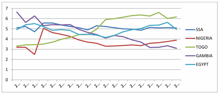
Figure 1 Total current health expenditure 2000-2018
Conflict of Interest
The authors declare no conflict of interest.
- World Health Organisation, “State of financing in the African region Systems”, World Health Organization. Regional Office for Africa, no. January, pp. 1–25, 2013.
- X. Weibo, B. Yimer, “The Effect of Healthcare Expenditure on the Health Outcomes in Sub-Saharan African Countries”, Asian Journal of Economics, Business and Accounting, vol. 12, no. 4, pp. 1–22, 2019, doi:10.9734/ajeba/2019/v12i430158.
- N. M. Odhiambo, “Health expenditure and economic growth in sub-Saharan Africa: an empirical investigation”, Development Studies Research, vol. 8, no. 1, pp. 73–81, 2021, doi:10.1080/21665095.2021.1892500.
- B. Yimer Ali, R. Moracha Ogeto, “Healthcare Expenditure and Economic Growth in Sub-Saharan Africa”, Asian Journal of Economics, Business and Accounting, vol. 13, no. 2, pp. 1–7, 2020, doi:10.9734/ajeba/2019/v13i230170.
- S. M. Piabuo, J. C. Tieguhong, “Health expenditure and economic growth – a review of the literature and an analysis between the economic community for central African states (CEMAC) and selected African countries”, Health Economics Review, vol. 7, no. 1, pp. 1–13, 2017, doi:10.1186/s13561-017-0159-1.
- M. O. F. Commerce, “The Determinants of Government Expenditure in South Africa by Glenda Maluleke”no. November, 2016.
- B. Aboubacar, D. Xu, “The Impact of Health Expenditure on the Economic Growth in Sub-Saharan Africa”, Theoretical Economics Letters, vol. 07, no. 03, pp. 615–622, 2017, doi:10.4236/tel.2017.73046.
- V. V Tarasova, V. E. Tarasov, “ECONOMIC GROWTH MODEL WITH CONSTANT PACE AND DYNAMIC MEMORY”vol. 2, no. 2, pp. 40–45, 2017, doi:10.20861/2304-2338-2017-84-001.
- E. F. Nwaolisa, “THE IMPACT OF GOVERNMENT EXPENDITURE ON NIGERIA ECONOMIC GROWTH : A FURTHER DISAGGREGATED APPROACH”vol. 5, no. 2, 2017.
- K. Tsaurai, “IS WAGNER ’ S THEORY RELEVANT IN EXPLAINING HEALTH EXPENDITURE DYNAMICS IN BOTSWANA ?”vol. 3, no. 4, pp. 107–115, 2014.
- O. E. Akpokerere, E. J. Ighoroje, “The Effect of Government Expenditure on Economic Growth in Nigeria : A Disaggregated Analysis from 1977 to 2009”vol. 4, no. 1, pp. 76–82, 2013.
- R. S. Juma, H. Ouyang, J. Cai, “The effect of government expenditure on economic growth : The case of Tanzania using VECM approach”vol. 9, no. 2, pp. 144–155, 2018.
- P. B. Frimpong, G. Adu, “Population Health and Economic Growth in Sub-Saharan Africa: A Panel Cointegration Analysis”, Journal of African Business, vol. 15, no. 1, pp. 36–48, 2014, doi:10.1080/15228916.2014.881227.
- S. Zaidi, K. Saidi, “Environmental pollution, health expenditure and economic growth in the Sub-Saharan Africa countries: Panel ARDL approach”, Sustainable Cities and Society, vol. 41, pp. 833–840, 2018, doi:10.1016/j.scs.2018.04.034.
No related articles were found.