Identification of Finite Impulse Response (FIR) filters refer to finding out the coefficients also known as the weights of its transfer function. Adaptive filtering using Least Mean Square (LMS) Algorithm is used to find the estimated weights of the transfer function, using ATMEGA16 processor. This method can be used to find the coefficients of complex resistive circuits. This is done by constantly comparing the FIR system with Adaptive filter until the difference signal is zero, both the systems are fed with same input signals.

1. Introduction

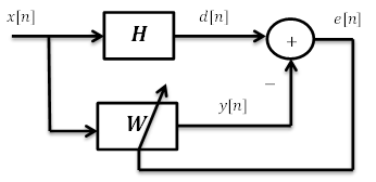
System Identification is the process of determining the attributes of the system by repetitive experimentation. Here, the system to be examined is a Finite Impulse Response (FIR) filter. If the Impulse response of a system is having finite number of coefficients such a system is called finite impulse response filter. A network consisting of only resistive components can be considered as a FIR filter having only one coefficient in its impulse response. The idea is to provide a linear model to the unknown system using adaptive filter that represents the best possible representation to the system to be identified, i.e., find the approximate weights of response (h[k]) of that particular system to impulse input[1-3]. Figure 1 shows block diagram of simple identification of system using LMS.

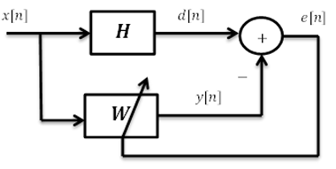
d[n]:Output of the system H for input signal x[n]
y[n]:Output of the Adaptive filter
e[n]:error function

2. Related Work

In [1], the author presented an identification of a system using stochastic gradient algorithm, which is known as least mean square algorithm. These filters are implemented using Digital Signal Processing (DSP), for increasing performance these are implemented using ASICs or FPGA. The main logic here is taking gradient descent for estimating a time varying signal. This will find min value and by way of taking increasing steps in negative direction of gradient. It is done in order to reduce error signal value.

Basically, using these two equations the unknown system is identified using LMS algorithm.

where µ is the main parameter which decides the efficiency of the adaptive output signal. We should make sure to keep it to desired value so that it will converge properly. The main reason for using LMS algorithm is that it is comparatively very simple to implement in both hardware as well software as it is computationally simple and efficiently uses memory.

In [2], author proposed comparative analysis of three commonly used adaptive filtering algorithms in System identification is they are Least Mean Square (LMS), Recursive Least Square (RLS) and normalized least mean square (NLMS) algorithms. LMS is computationally simple than the other two, NLMS is its normalized form and RLS is a complex but efficient algorithm.

The LMS adaptive filter updating equations are similar to the above paper, in NLMS the major challenge in finding the appropriate value of the step size is overcome by normalizing the input and its updating equation is as shown,

The RLS is a recursive algorithm which has good convergence but computationally complex moreover, it requires predefined conditions and information to update the estimation.

In [3], the author has presented the LMS algorithm which is improved by an approach called LMS-GA. The genetic searching methodology is integrated with LMS algorithm to speed the process and reduce time in this algorithm. This algorithm also preserves the simplicity of LMS algorithm, has fewer computation and has fast convergence rate. The LMS-GA algorithm out performs the basic LMS algorithm.

In [4], the author has presented a method to overcome the problem of decrease in performance when signal to interference ratio (SIR) is low this overcomes by the use of varing step size in Least mean square method. It provides a different non linear relationship between step factor and  error of adaptive system. The relationship is written as represented in eq. (4). This algorithm is not sensitive to interference and has better performance when compared to the commonly used LMS algorithm when the SNR is less.

In [5], the author has proposed an adaptive filtering method when the system is scattered. This method applies l1 relaxation, to enhance LMS type adaptive filters performances two new algorithms are introduced, they are the zero-attracting least mean square (ZA-LMS) and the reweighted zero-attracting least mean square (RZA-LMS). By combining a l1 norm penalty in the coefficients into the quadratic Least mean square cost function ZA-LMS can be obtained. To better the filtering ability further RZA-LMS is designed utilizing a re-weighted ZA, numerically RZA-LMS’s performance is better than ZA-LMS. Both algorithms are compared in performance with the typical LMS algorithm which results in improved ZA-LMS and RA-LMS in comparison to the typical LMS both in steady-state performance and transient performance when the system is scattered, it also shows the reduced MSE from ZA-LMS algorithm.

In [6], the author has presented LMS algorithm with variable step size along with a functional relationship between the difference signal and step-size which is nonlinear in nature. A hop parameter (αn) is used in this algorithm to remove the disturbances of independent noise by varying the step-size. This algorithm also presents a similar method that is based on the Sigmoid function (SVSLMS) whose size of step is high although the difference signal is approximately to zero. The system formula of SVSLMS algorithm is represented in eq. (5).

The simulation results run on a Computer confirms that the method is better compared to the previous algorithms in performance, the convergence properties are better at the beginning of adaptation while establishing very less eventual miss-adjustment.

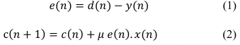
In [7], the author has proposed two new versatile adaptive calculation methods, in particular Prominent subspace least mean square (PS-LMS) and PS-LMS+. This helps for quicker estimation of unknown models, which are scattered in transfer domain. PS-LMS calculations are valuable for quick recognizable proof of varying unknown systems and furthermore enhances the union speed of standard Least mean square calculation if the system to be found is scattered and has long impulse response. To decrease the error PS-LMS+ adaptive method was introduced as shown in Figure 2. Performances of PS-LMS and PS-LMS+ algorithms are compared with typical algorithms such as LMS, RLS, PN-LMS, μ-law PN-LMS adaptive methods by conducting experiments. The outcome furnishes a quicker speed of convergence with compromise of marginally higher computational intricacy compared to typical LMS algorithm.

In [8], the author has explained NLMS (normalized least mean square) algorithm whose behaviour is same as that of Least mean square-SAS algorithm. In NLMS algorithm the gradient estimation error is used, which will be present in normal adaptive process, this acts as perturbing noise. NLMS algorithm is easy and simple, which increases the computational speed in comparison to LMS algorithm which has comparatively small step size. In LMS-SAS Edmonson uses estimated gradient vector for finding perturbing noise. Author has shown that NLMS is better when compared to LMS-SAS algorithm. And efficiency is greater compare to GLMS algorithm because it does not require any cooling schedule.

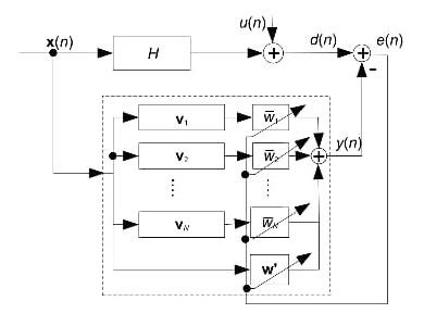
In [9], the author has compared different methods to find the unknown system and other distinct PI controllers are developed to identify response of system. To identify the existence of different model parameters several system identification models are utilized and accuracy of the model is most vital step to design efficiently. The states of the linear system can be estimated using the Kalman filter (KF), it comprises of two major steps first prediction step and then correction steps. Non-linearity in the state space model can be seen as a result of extension and Extended Kalman Filter (EKF) is used for this identification, which is shown in Figure 3. Parameters of the system and its internal states can be estimated efficiently using extended Kalman filter.

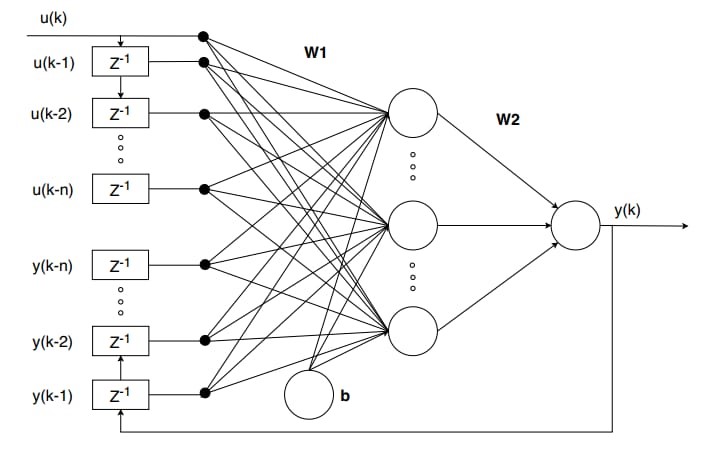
Nonlinear Autoregressive Exogenous Model (NARX) is a multi-layer recurrent perceptron neural system network, which can be utilized as a black-box identifying technique. Both parallel and series-parallel architecture can be seen in NARX. The simple block diagram is shown in Figure 4. The major benefit of this estimation method is that, it is not necessary to have information about the system to be found and it is effective for both linear and nonlinear systems. A high convergence rate can be obtained in all the other methods other than the LMS. The MSE comparison between LMS and NARX gives mid accuracy in comparison to RLS and EKF. Highest precision can be realized using EKF but this result in increase in cost and complexity.

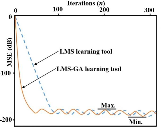
In [10], the author has proposed a simple way of using adaptive IIR filter in system identification. The improved genetic search approach of Least Mean Square (LMS) algorithm that is Least Mean Square-Genetic Algorithm (LMS-GA) helps in searching the multi-model error surface of the IIR filter. This helps in avoiding local minima and in finding the optimal weight vector. Genetic Algorithm (GA) is an optimization approach used in applications of vast, nonlinear and potentially discrete systems. In GA, a population of strings called chromosomes which represent the candidate solutions to an optimization problem is evolved to a better population. GA as the maximization of fitness function is given by,

here the cost function to be minimized is represented as f(t).  The cost function f(t) is taken as the Mean Square Error (MSE) in adaptive filtering which is given by

here te represents the size of window along which errors are accumulated and y_j(n) is the estimated output for the jth set of estimated parameters. Graph of MSE versus Iterations is shown in below Figure 5.

To understand parameters of the digital filters (FIR and IIR) and to minimize error signal the adaptive algorithms LMS and LMS-GA are adopted. The characteristics and the simplicity of the standard LMS learning algorithm can be preserved with comparatively fewer computations and fast convergence rate using LMS-GA algorithm [11-15].

3. Methodology

The methodology of the system is demonstrated in Figure 6. The unknown FIR system to be recognized and the adaptive system both are fed with the same input signal. For the input a White noise generator is used which generates white noise signal.

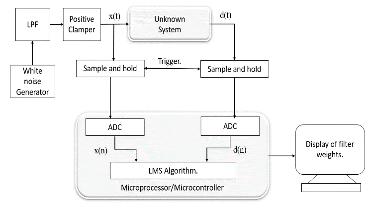
This is passed to a low pass filter to attenuate higher frequencies as the speed of the sampling in the ATMEGA16 is limited. Then, this signal clamped using a clamper circuit to eliminate negative components in the signal. Since the applied signal is Analog and the adaptive filter used is a digital filter, the input signal that is fed to the adaptive filter and the output from the unknown FIR filter must be passed through a Sample and hold circuit. Both the sampling processes should be triggered simultaneously. The output from both the FIR system and the adaptive filter is compared to obtain the difference signal. This difference signal is basis for further calculations. This error signal is used update the adaptive filter coefficients. This process continues until the difference between the signals is negligible. The entire process of the LMS algorithm is implemented in the ATMEGA16 processor. Then the output coefficients i.e., the impulse response coefficients of the FIR filter are displayed on the screen using Putty.

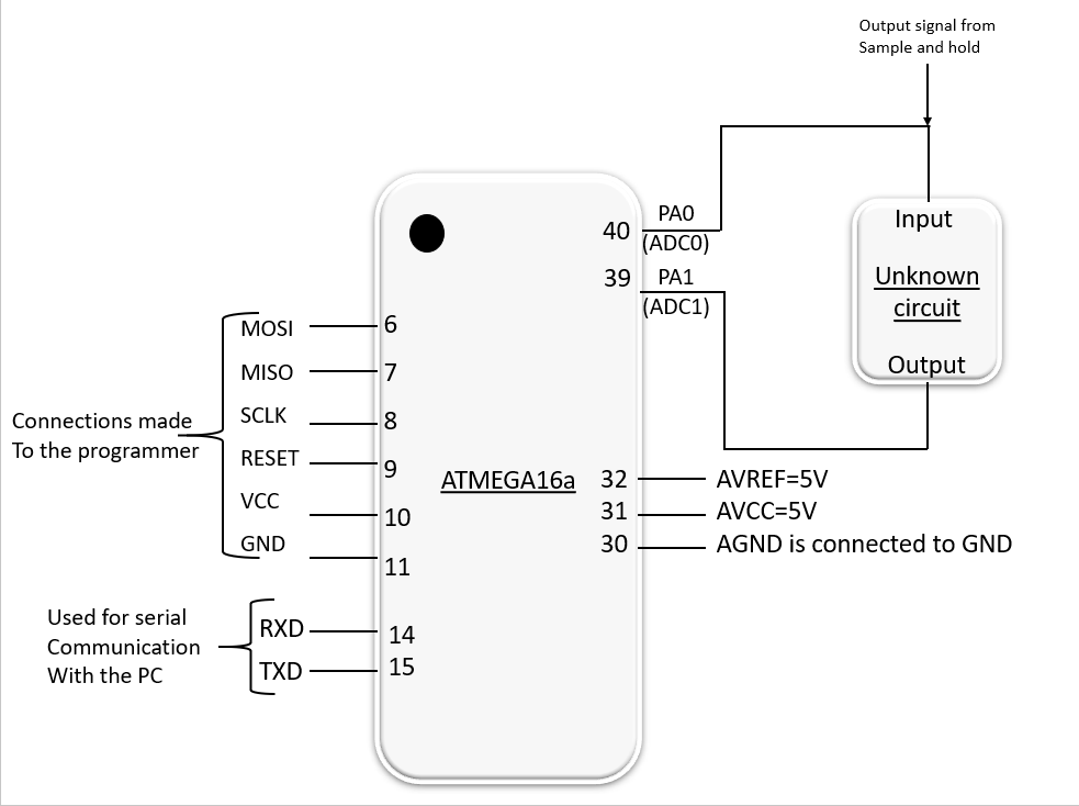
3.1. ATMEGA16 Interconnection

Microcontroller is the most important component of this system. Here, we have used ATMEGA16 as our microcontroller and its interconnections and pins used for this system are shown in Figure 7.

3.2.  Work contribution and Working of LMS Algorithm

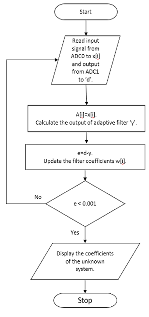
As discussed earlier the adaptive filtering algorithm adopted is LMS. The working of LMS code in the ATMEGA16 is as shown in the flowchart Figure 8. The steps involved are:

• Read the values, one from the input given to the unknown system into the ADC channel0 further stores it into x[i] and another from output of the unknown system into the ADC channel1 and store it in the variable d.

• Assume A[i]=x[i], where a[i] as the input to adaptive filter.
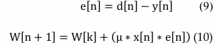
• find the adaptive filter output ‘y’ using formula in (8)

• Calculate error using (9) and update the coefficients of the filter using (10).

• Check if error is less than 0.001, if yes display the coefficients of the unknown undefined system and stops the method else repeat the similar process until the condition is satisfied.

4. Results

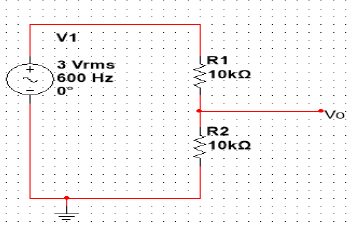
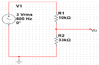
The FIR circuit is tested with resistive circuit. The output obtained was reduced to half. This half value will be the filter coefficient (weights). Below shows the Figure 9 of simple FIR resistive circuit with same resistor value.

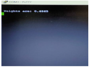
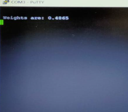
Using puTTy the output was read from TTL converter. The weighted value is approximately equal to 0.5 is as shown in Figure 10.

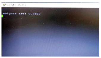
To understand parameters of the digital filters (FIR and IIR) and to minimize error signal the adaptive algorithms LMS and LMS-GA are adopted. The characteristics and the simplicity of the standard LMS learning algorithm can be preserved with comparatively fewer computations and fast convergence rate using LMS-GA algorithm. The model is also determined for different FIR circuit and verified for accurate results. Figure 11 shows the two resistive circuit having different value. LMS adaptive filtering algorithm is implemented but it is not most accurate. In order to overcome this, different adaptive techniques of filtering can be realized. NLMS algorithm in which the input is normalized, LMS-GA which uses a genetic search approach, LMS with varying step size and other such algorithms have been developed. The obtained results were approximately equal to 0.76 as shown in Figure 12. For more accurate results we need to use RLS. But RLS is computationally complex and the estimate is more accurate to the unknown system.  The performance comparison of LMS, NLMS and RLS is tabulated in Table 1.

Table 1: Performance Comparison of LMS, NLMS & RLS Algorithms

5. Conclusion

The Adaptive scheme is used to understand the FIR filters parameters, which is the weights of unknown undefined system. There are many adaptive techniques which are realized to determine the unknown function. The simpler way for understanding and configurable for hardware and software is LMS algorithm. But for higher input accuracy and performance is very hard to predict. In order to overcome this problem many other algorithms are used such as NLMS, RLS, LMS-GA. Hence the choice of algorithm can be made based on the application, for example for an application involving the estimate to be highly accurate with cost and computationally complexity not being an issue RLS algorithm can be used, but for applications where approximate result is sufficient keeping the complexity simple then LMS algorithm is preferred. Therefore, for laboratory application where the accuracy is not an issue but requires simplicity in the LMS algorithm is used.

1. Irina Dorean, Marina Topa, Botond Sandor Kirei and Erwin Szopos, “Interdisciplinarity in Engineering” Scientific International Conference, TG.MURES – ROMÂNIA, 15-16 November 2007.
2. S. A. Ghauri and M. F. Sohail, “System identification using LMS, NLMS and RLS,” 2013 IEEE Student Conference on Research and Developement, 2013, pp. 65-69, doi: 10.1109/SCOReD.2013.7002542.
3. Ibraheem, Ibraheem Kasim. “Adaptive System Identification Using LMS Algorithm Integrated with Evolutionary Computation.” arXiv preprint arXiv: 1806.01782 (2018).
4. T. Jia, Z. J. shu and W. Jie, “An Improved Variable Step Size LMS Adaptive Filtering Algorithm and Its Analysis,” 2006 International Conference on Communication Technology, 2006, pp. 1-4, doi: 10.1109/ICCT.2006.341916.
5. Yilun Chen, Y. Gu and A. O. Hero, “Sparse LMS for system identification,” 2009 IEEE International Conference on Acoustics, Speech and Signal Processing, 2009, pp. 3125-3128, doi: 10.1109/ICASSP.2009.4960286.
6. Q. Yan-Bin, M. Fan-Gang and G. Lei, “A New Variable Step Size LMS Adaptive Filtering Algorithm,” 2007 IEEE International Symposium on Industrial Electronics, 2007, pp. 1601-1605, doi: 10.1109/ISIE.2007.4374843.
7. R. Yu, Y. Song and S. Rahardja, “LMS in prominent system subspace for fast system identification,” 2012 IEEE Statistical Signal Processing Workshop (SSP), 2012, pp. 209-212, doi: 10.1109/SSP.2012.6319662.
8. Ching-An Lai, “NLMS algorithm with decreasing step size for adaptive IIR filters,” Signal Processing, Volume 82, Issue 10, October 2002, pp. 1305–1316, https://doi.org/10.1016/S0165-1684(02)00275-X.
9. G. Akgün, H. u. Hasan Khan, M. Hebaish and D. Gohringer, “System Identification using LMS, RLS, EKF and Neural Network,” 2019 IEEE International Conference on Vehicular Electronics and Safety (ICVES), 2019, pp. 1-6, doi:
10. 1109/ICVES.2019.8906339.
    10. Ibraheem Kasim Ibraheem, Adaptive IIR and FIR Filtering using Evolutionary LMS Algorithm in View of System Identification, International Journal of Computer Applications (0975 – 8887), Volume 182 – No. 11, August 2018.
11. S. C. Douglas, “Analysis of the multiple-error and block least-mean-square adaptive algorithms,” in IEEE Transactions on Circuits and Systems II: Analog and Digital Signal Processing, vol. 42, no. 2, pp. 92-101, Feb. 1995, doi: 10.1109/82.365348.
12. Geun-Taek Ryu, Dong-Won Kim, Jung-Go Choe, Dae-Sung Kim and Hyeon-Deok Bae, “Adaptive system identification using fuzzy inference based LMS algorithm,” Proceedings of Third International Conference on Signal Processing (ICSP’96), 1996, pp. 587-590 vol.1, doi: 10.1109/ICSIGP.1996.567332.
13. E. Szopos, M. Topa and N. Toma, “System identification with adaptive algorithms,” 2005 IEEE 7th CAS Symposium on Emerging Technologies: Circuits and Systems for 4G Mobile Wireless Communications, 2005, pp. 64-67, doi: 10.1109/EMRTW.2005.195681.
14. M. Nakamoto, N. Shimizu and T. Yamamoto, “A system identification approach for design of IIR digital filters,” IECON 2013 – 39th Annual Conference of the IEEE Industrial Electronics Society, 2013, pp. 2360-2365, doi: 10.1109/IECON.2013.6699500.
15. Archana Sarangi, Shubhendu kumar Sarangi, Siba Prasada Panigrahi, “An approach to identification of unknown IIR systems using crossover cat swarm optimization,” Perspectives in Science, Volume 8, 2016, Pages 301-303, Doi: 10.1016/j.pisc.2016.04.059.

Citations by Dimensions

Citations by PlumX

Crossref Citations

This paper is currently not cited.

No. of Downloads per Month

No. of Downloads per Country