Pressure (BP) waveform is a result of the response of the arteries to the blood ejectionproduced by tant indicator of the state of the cardiovascular system. Currently, its measurement is performed invasively in critically ill patients who need a continuous and real time monitoring of their treatment response, however, it is possible to measure the BP, continuously and non-invasively, in non-critical patients to detect, monitor and control possible hypertensive events. Nevertheless, current non-invasive techniques can cause discomfort in patients and they are not used in critically ill patients. Consequently, non-Invasive and minimally-Intrusive methodologies (nImI) are required to estimate BP and its waveform. In the current study, the performance of machine learning algorithms, specifically the Extreme Learning Machine (ELM) algorithm, is evaluated to estimate both Blood Pressure and its waveform from the Photoplethysmography (PPG) signal and its first derivative’s (VPG) waveforms. A total of 15 healthy volunteers participated in this study. They performed two handgrips, which is isometric maneuver to induce controlled BP rises. The first handgrip is used to train ELM and the second handgrip is used to test the ELM. Our results show that there are high correlation performances (0.98) between the estimated and measured BP waveforms, and a relative error of 3.3 1.4%. An arterial volume-clamp at the middle finger is used as the gold-standard measurement. Meanwhile, BP extreme values estimations, Systolic BP (SBP) and Diastolic BP (DBP), are also performed. ELMs have a performance with an average RMSE of 5.9 ± 2.7 mmHG f and 4.8 ± 2.0 mmHg for DBP and, an average relative error of 5.0 ± 2.7% for SBP and 7.0 ± 4.0% for DBP.

1. Introduction

Arterial Hypertension (AHT) is a deadly disease that affects 70 million in the USA and 1,000 million people worldwide. AHT is still the most common risk factor and it is responsible for 54% of strokes and 47% of ischemic heart diseases worldwide [1].

Invasive methods have been used for Blood Pressure (BP) monitoring in critically ill patients for more than 50 years because they facilitate rapid diagnoses and allow us to monitor treatment responses in real-time. Medical procedures are said to be invasive when they require that the external natural protective barriers of the body, such as skin, are pierced, either through cuts or by inserting a medical device into the body. These measurements are more accurate than non-invasive methods because they introduce a cannula in the arterial system to measure BP directly from the artery [2]. Nevertheless, these methods require medical supervision to avoid injuries in the patient.

Medical devices are said to be intrusive when the procedures generate discomfort in patients, decreasing the adherence to the procedure. In particular, non-invasive procedures to measure BP, such as ambulatory blood pressure monitoring, are perceived by the patients as intrusive, the procedure is frequently abandoned, and the detection, monitoring and control of AHT remain elusive [3].

Although the morphology and detail of the arterial pressure waveform can provide useful diagnostic information, modern physicians pay little attention to it [4]. This results in an important waste of a potential diagnostic aid whose usefulness was first recognised over 100 years ago [5]. Ma- homed used sphygmography in his studies to analyse the arterial pressure waveform, a technology with levers hooked to a scale-pan in which weights were placed to determine the amount of external pressure needed to stop blood flow in the radial artery [6]. According to [7], sphygmography lapsed with the introduction of the cuff sphygmomanometer, which only provides the extreme values of the arterial pressure pulse.

Although the measurement of the difference between systolic and diastolic pressures from a single pulse has been used to assess arterial stiffness and cardiovascular risk [8], important additional information is contained within the pressure waveform [9], such as augmentation index, left ventricular workload, cardiac output and, in a lower level, arterial stiffness [10]. Consequently, the use of pulse wave analysis may serve as a guide for physicians when making choices about blood pressure treatment in prehypertensive or hypertensive patients [11].

The pressure wave is generated by the contraction of the left ventricle, which imparts its contractile energy on the blood mass that it contains, raising the pressure to overcome the diastolic pressure in the aorta to open the aortic valve, ejecting the blood and deforming the radius of the aorta lumen [9]. As the ventricle ejects the blood mass into the aorta with each systole, it creates a pulsatile pressure and flow. The pressure wavefront is propagated to most of the peripheral arteries at 8 to 10 m/s, although the blood that leaves the left ventricle takes several cardiac cycles to reach the same distance [7].

The acronym nImI is proposed to summarise a concept that could be applied to medical devices—a device would be nImI if and only if it is non-invasive and it is minimally- intrusive. Non-invasive devices are able to monitor the arterial pressure waveform, such as those based on the volume clamp [12] technique (FINAPRES, CNAP, etc.) and those based in applanation tonometry techniques. Both of these techniques measure blood pressure waveform in a specific point of the body and they then reconstruct brachial and aortic BP waveforms, respectively, with validated algo- rithms. Nevertheless, analysis from the brachial pressure waveform is not considered to be a suitable indicator for car- diovascular risks [13] and applanation tonometry is not yet a reliable tool to monitor pressure waveform in long-term clinical interventions [14].

Photoplethysmography (PPG) has been studied to estimate and monitor BP non-invasively, measuring the Pulse Transit Time (PTT) and, therefore, the Pulse Wave Velocity (PWV), which are directly related to BP. PTT can be easily measured from a PPG waveform, and it is less expensive and cumbersome than the previously described devices [15]. Nevertheless, the normal use of PPG carries artifacts that interfere with a proper signal preprocessing [16]. However, new clinical applications have been proposed that are sup- ported by computational solutions [17] and novel wearable devices such as smartwatches [18].

The relationship between the PTT and BP is so strong that a device which estimates BP from PTT was patented at the beginning of the 21st century, where two parameters were consider for each subject [19]. Furthermore, the correlation between the BP and PTT has been proven under exercise and drug administration conditions [20]. In previous works by [21] and [22], new approaches were tested to relate PPG and BP. In the first, machine learning has been used to classify PPG waveforms corresponding to high and normal BP in healthy subjects. In the second, PPG is fitted to the finger Arterial Pressure (fiAP).

Recently, some authors have proposed the application of machine learning methods to estimate the BP waveform (see [23]–[25]). In [23], the author proposed an ensemble of support vector regression SVR models to predict the BP [24] have applied SVR combined with genetic algorithms to estimate systolic BP and diastolic BP. In [25], the author pro- posed the Deep Boltzmann machine to estimate the blood pressure.

The main goal of this work is to validate the mExtreme Learning Machine (ELM) as a model that relates the PPG to fiAP and brachial reconstructed Blood Pressure (reBP) waveforms. This work is structured as follows. In section 2, we introduce the Extreme Learning Machine, the main model used in this article. In section 3, we describe the data acquisition process, the signal processing process and the ELM architectures. The performance results are given in section 4 and we give a discussion in section 5. Finally, some concluding remarks are given in section 6.

2. Theoretical Framework: Extreme Learning Machine (ELM)

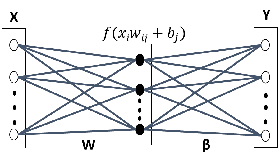
ELM [26] has been proposed for training single hidden layer Feedforward Neural Networks (SLFN) [27], as shown in Figure 1. Feedforward Neural Networks (FNN) have been widely used since the introduction of the back propagation algorithm [28], which is essentially a first order gradient method for parameter optimisation and, therefore, has slow convergence problems. In addition, ELM has much lower computational complexity and is particularly attractive for high dimensional and large data applications. In this paper, the ELM algorithm is used for nImI BP estimates from three different inputs PPG and VPG signals, and for a combination of them.

The main characteristic of ELM is that once the input weights and biases, from input to the hidden layer, are ran- domly defined, they are not further modified in the learning process. Consequently, ELM has a very short training time. Furthermore, ELM is remarkably efficient and tends to reach global optimum [29]. Various extensions have been made to the original ELM model to make it more efficient and suitable for specific applications [26].

These types of algorithms are suitable for the new era of big data processing, where large amount of data need to be processed in short time. ELM, as a learning technique, is able to provides efficient unified solutions to generalised FNN, including single and multi-hidden layers neural net- work. This algorithm has both universal approximation and classification capabilities [30].

The input vector is mapped to L-dimensional ELM random feature space, let x_i x₁, x₂, …, x_d be the input vector shown in Figure 1, x_i ∈ χ ⊆ R^d and T t₁, t₂, …, t_N the targets values, (i 1, 2, …, N). The parameters of the j-th hidden node are w _j corresponding to the weight vector connecting the j– th hidden node to the input nodes, where w _j w_{1 j}, w_{2 j}, …, w_{L j} and b _j, corresponding to the threshold or bias. ( j 1, 2, …, L) and L is the number of nodes in the hidden layer. These con- nections are randomly assigned and they remain unchanged during the learning process.

The k-th output function of ELM for generalised SLFN is:

$$y_k \mathbf{x}_i = \sum_{j=1}^{L} \beta_{jk} h_j(\mathbf{w}_j, b_j, \mathbf{x}_i) = \mathbf{h} \mathbf{x}_i \beta_k, \quad i = 1, \ldots, N,\; k = 1, \ldots, K \tag{1}$$

where the vector β_k β_1k, …β_Lk^T contains the weights between the hidden nodes and the k-th output node. H is the hidden layer output matrix of the neural network, where the i-th column of H is the output of the j-th hidden node with respect to the input x_i:

$$\mathbf{H} = \left( \begin{array}{ccc}
f_{\mathbf{w}_1, b_1, \mathbf{x}_1} & \cdots & f_{\mathbf{w}_L, b_L, \mathbf{x}_1} \\
\cdots & \cdots & \cdots \\
f_{\mathbf{w}_1, b_1, \mathbf{x}_N} & \cdots & f_{\mathbf{w}_L, b_L, \mathbf{x}_N}
\end{array} \right) \tag{2}$$

where f w _j, b _j, x_i is an activation function that satisfies the ELM universal approximation capability theorem [26]. In this paper, the threshold function was used:

$$f_{\mathbf{w}, b, \mathbf{x}} = \left\{ \begin{array}{ll}
1, & \text{if } \mathbf{w} \cdot \mathbf{x} + b \leq 0 \\
0, & \text{otherwise}
\end{array} \right. \tag{3}$$

The ELM learning process consists in solving matrix equation on vector beta:

$$\mathbf{H} \boldsymbol{\beta} \mathbf{T} \tag{4}$$

In theory, if the number of the L neurons in the hidden layer is equal to the number of the possible samples that constitute a problem and, furthermore, H is invertible, then the solution for β will be found multiplying by H⁻¹ at the left-hand of the equation and solving it by linear least squares method [29]:

$$\mathbf{H}^{-1} \mathbf{H} \boldsymbol{\beta} \ \mathbf{H}^{-1} \mathbf{T} \rightarrow \boldsymbol{\beta} \ \mathbf{H}^{-1} \mathbf{T} \tag{5}$$

Nevertheless, the vector H will generally not be square and invertible and, for this reason, the values of β will be:

$$\boldsymbol{\beta} \ \mathbf{H}^{\dagger} \mathbf{T} \tag{6}$$

where H^† is the generalised Monroe-Penrose inverse of the matrix H and, therefore, the values of weights connecting the hidden layer with output neurons layer (β) can be found multiplying it by the T vector [31], [29] and [26].

3. Materials and Methods

In this paper, new methodologies are tested to estimate either fiAP and reBP waveforms or SBP and DBP values from PPG. Signals from 15 healthy subjects are recorded and ELM machine learning algorithms are trained to do these BP estimations for each subject.

The required cardiovascular signal acquisition is per- formed in each subject. The subjects are asked to answer a questionnaire that is adapted from the AHT Clinical Guide of the Chilean Ministry of Health and to sign an informed consent that is approved by Bioethics Institutional Com- mittee for Human Beings Research of the Universidad de Valparaíso (CIBI-SH UV for its acronym in Spanish), accept- ing to perform the clinical essay.

BP is measured with an oscillometric technique in each subject twice before performing the clinical essay to ensure that the subjects do not have a SBP greater than 140 mmHg or a DBP greater than 90 mmHg. If they declare that they have a cardiovascular disease, then they are excluded from the study.

3.1. The Subjects’ Characteristics

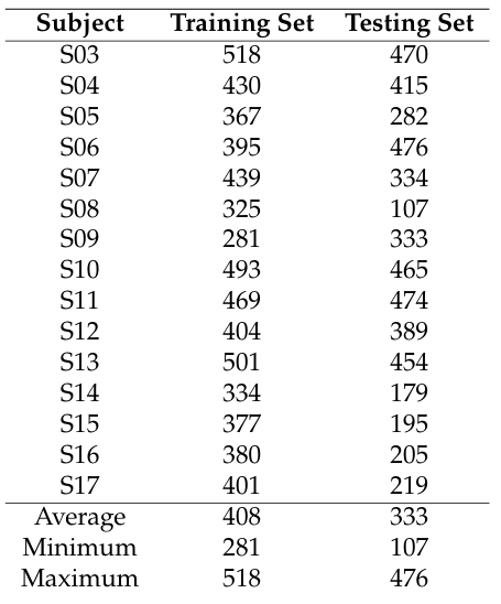
Table 1 shows the characteristics of the 15 healthy subjects that participated in this study. Data from these subjects can be found in [32], within the Readme file in section “Get- ting the Dataset” of “About nImI”. Column 2 shows the corresponding code name for each subject of column 1.

In this study, the data were gathered from 10 females and 5 men with a mean age of 31.3 ± 10.8 years old. The youngest subject is 18 years old and the oldest is 50 years old. As is explained on the website, different essays that are performed by volunteers in the project and different configurations for data recordings are used, depending on the essay. Consequently, only those subjects that performed a particular essay are studied in this article. Each subject performs an isometric handgrip maneuver twice to induce BP rises in SBP and DBP while the signals are recorded.

Two oscillometric BP measurements are performed in each subject to obtain their SBP and DBP values for two reason. The main reason is to corroborate that the subject is normotensive and can perform the clinical essay and the second reason is to calibrate the Finapres NOVA.

3.2. Data Acquisition

A detailed description of the data acquisition, signal pro- cessing and segmentation is given in [22]. Briefly, PPG and ECG signals are recorded, respectively, in the bandwidth from DC to 10 Hz and from 0.3 to 35 Hz using the BIOPAC system. The fiAP waveform is recorded using Finapres NOVA (FN) of [33]. The brachial blood pressure waveform (reBP) is reconstructed by FN from fiAP and its extreme values correspond to SBP and DBP. The signals are sampled at 200 Hz.

Once the signals have started to be recorded, the hand- grip maneuver is performed after a resting time of 10 min- utes. During this period, the FN is calibrated (with the two oscillometric BP measurements shown in Table 1) and the subject can relax and receive instructions about the handgrip maneuver. Then, the subject must press a device in a sustained manner during a standardised time. The maneuver is performed twice, with a resting time of 10 minutes between them.

Table 1: Characteristics of the subjects (S) participating in the study, which shows their ages, sex and their two oscillometric BP measurements (M1 and M2) performed to obtain DBP and SBP mmHg.

Subjects Characteristics

S       Code      AGE     SEX          DBP               SBP

            Name                                 M1     M2     M1     M2

1         S03          18           F          69       78      107     120

2         S04          49          M         81      100     129     161

3         S05          29           F          78       84      117     129

4         S06          28          M         63       92      111     149

5         S07          40           F          73       93      106     141

6         S08          33           F          81       94      130     139

7         S09          50          M         61      109     115     207

8         S10          45           F          63       69       90      100

9         S11          26           F          59       71      102     113

10        S12          26          M         64      102     120     155

11        S13          38           F          75       81      122     134

12        S14          20           F          62       88      117     154

13        S15          29          M         76      108     122     170

14        S16          19           F          60       79      108     138

 15        S17          20           F          72       85      115     121

During each handgrip, the subject steadily grips a cuff with his or her deft hand for 3 minutes. The pressure over the cuff is at one third of the subject’s maximal strength. After the 3 minutes, the subject releases the cuff and rests for three additional minutes. Afterwards the recording is stopped. These essays were conducted at the School of Biomedical Engineering (EICB), Faculty of Engineering, Universidad de Valparaiso (Chile).

3.3. Photoplethysmography signal processing

Photoplethysmography (PPG) is sensitive to thermal changes, movements and respiration [16]. Consequently, the raw PPG is processed with two FIR filters (detailed description in [22]). Later, PPG first derivative, or velocity of PPG, VPG, is evaluated using a five point stencil algorithm. PPG is segmented beat to beat using ECG and it is then processed to extract the sections that have suffered interference from spiky blocking noise.

3.3.1. Pre-processing of the PPG

The PPG is preprocessed with two symmetric Finite Impulse Response (FIR) filters of order 17 and 799. The low order FIR low passes the signal at 6.5 Hz, smoothing the PPG and decreasing energy in quantisation error frequency band. The high order FIR high passes the signal at 0.2 Hz, stabilis- ing PPG’s DC component. VPG is calculated after the two FIR filters have been applied. It is performed with five point stencils (7) instead of the more conventional L’Hopital rule, which is known to produce noisy derivatives.

$$yn = \frac{-xn \cdot 2 \cdot 8xn \cdot (1 – 8xn – 1) \cdot (xn – 2)}{0.06} \tag{7}$$

3.3.2. PPG Signal Segmentation

Segmentation of PPG, VPG, fiAP and reBP during each heartbeat is needed to estimate fiAP and reBP waveform, and their BP values beat to beat.

A modified Pan-Tompkins Algorithm (PTA) [34], is used to detect R waves from ECG and to segment each cardiac cycle, which is the unit of study in this work. To accomplish this, the PTA’s band-pass filter in cascade with a Continuous Wavelet Transform (CWT) with a Mexican-Hat wavelet was applied. From CWT’s results, a threshold is established at 30% of the maximum amplitude in a R wave of the signal, which is chosen arbitrarily. Furthermore, a refractory time of 0.3 seconds is established [35], which represents the minimal period before the next QRS complex appears.

3.3.3. Noisy PPG Extraction

While PPG is transmitted from the sensor module to the Biopac system, an algorithm is implemented to detect and remove the PPG segments that have suffered interference from blocking noise [22] if a spiky communication interruption occurs and the signal is blocked. The unaffected segments are isolated and saved.

3.4. Signal Normalisation

Signals are normalised in amplitude and in time duration, or period. Period normalisation is necessary because a fixed number of inputs neurons are needed to train the ELM algorithms. Due to heart rate variability, each heartbeat has a different period and this results in a different numbers of samples in each. Consequently, 180 samples (0.9 seconds) are considered for each heartbeat.

Amplitude is normalised to estimate BP only using PPG and VPG waveforms and not their extreme values. Normalisation is applied on each signal by:

$$\mathbf{x}_i = \frac{\mathbf{x}_i – \min x_i}{\max x_i – \min x_i} \tag{8}$$

where x_i is the normalised signal.

3.5. Derivative Approaches

The standard terminology for photoplethysmogram signals presented in [36] is used in this paper. VPG and the second derivative of PPG (APG) have been studied in relation with Blood Pressure in [37].

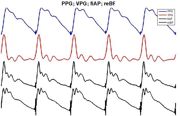
Figure 2 shows an example of PPG (blue), its first deriva- tive (red) and an example of the corresponding fiAP and reBP waveform for each heartbeat in black. In previous work [22], the relationship between PPG and fiAP has been studied in four subjects with two different approaches. The first approach is a Linear Combination of Derivatives (LCD):

$$LCD^i \quad \alpha PPG^i \quad 1 – \alpha PPG^{i1} \tag{9}$$

where PPG^k is the k^th order temporal derivative of the PPG, and α is a single parameter to fit PPG to fiAP and if LCD LCD⁰ then:

$$LCD \quad \alpha PPG \quad 1 – \alpha VPG. \tag{10}$$

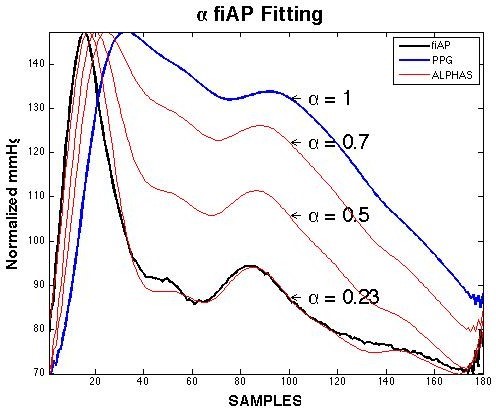
As shown in Figure 3, by modifying α, the PPG signal (blue) can be fitted in the fiAP signal (black), normalising the LCD result and “de-normalising” it within the BP extreme values of fiAP. Nevertheless, even though the fitting shows a strong relationship between these two signals, it does not have an estimate value because α for the best fit must be evaluated from each PPG waveform using its respective fiAP waveform. In [38], we have introduced a fractional derivative method applied to the PPG to obtain the fiAP signal. In this study, machine learning is used to estimate the fiAP and reBP waveform from different combinations of PPG and VPG waveforms.

3.6. ELM Training and Testing Sets to estimate BP

Each subject performs the handgrip maneuver twice. The signals from the first recording are used as the training set and the signals from the second recording are used as the testing set. 

Different ELMs are trained in each subject to estimate different targets: fiAP, reBP and the pair SBP/DBP. Fur- thermore, three ELMs are trained per target, with different inputs vectors: PPG, VPG and a modular combination of them. In summary, nine ELM algorithms are trained per subject.

To compensate the loss of physiological information produced by signals segmentation and normalisation, the estimation of SBP/DBP includes a second input vector mod- ule for each ELM network. This module has two input neurons, one with Pulse Transit Time (PTT) and the other with the Heart Rate (HR) of the corresponding signal’s heartbeat.

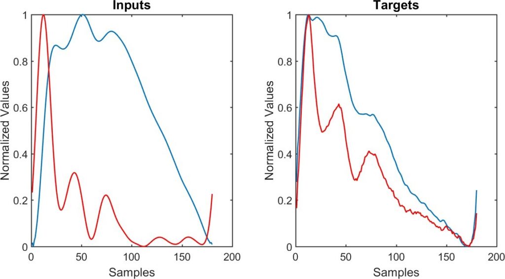
Figure 4 shows an example of the input and target wave- forms. On the left-hand, the PPG signal (blue) and VPG signal (red) are illustrated. On the right-hand, the fiAP signal (blue) and reBP signal (black) are illustrated.

It is important to mention that, only normalised wave- forms are considered to estimate fiAP and reBP. Thereafter, ELM outputs are denormalised into SBP and DBP values of the corresponding fiAP or reBP waveform and the results are then evaluated.

3.7. ELM Architectures

Two main approaches are used, depending on whether BP waveforms or systolic and diastolic values are to be estimated.

3.7.1. Approach 1: Finger and Brachial BP Waveform Estimates

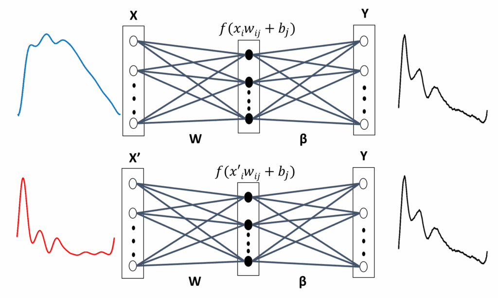
Both fiAP and reBP waveform estimation use similar ELM architectures, only the target vector is changed. Conse- quently, the following explanation applies to estimate fiAP or reBP. Architectures illustrated in Figures 5 and 6 are used to estimate either fiAP or reBP.

As mentioned, three types of input vectors—PPG, VPG and combination of them—are used to train ELM algorithms to estimate fiAP or reBP waveform. ELM with either PPG or VPG as input vector use the architecture illustrated in Fig- ure 5, which will referred as ELM1 and ELM2, respectively. ELM1 or ELM2’s output vector is obtained in (11):

$$y_k \; g\left( \sum_{j1}^{M} f\left( \sum_{i1}^{N} w_{ji} x_i + b_j \right) \beta_{kj} \right) \tag{11}$$

where k 1, 2, …, N, y_k is the k^th value of the output vector, g is a linear activation function, f correspond a hardlim activation function, and X x₁, x₂, …, x_N is the PPG or the VPG input vector.

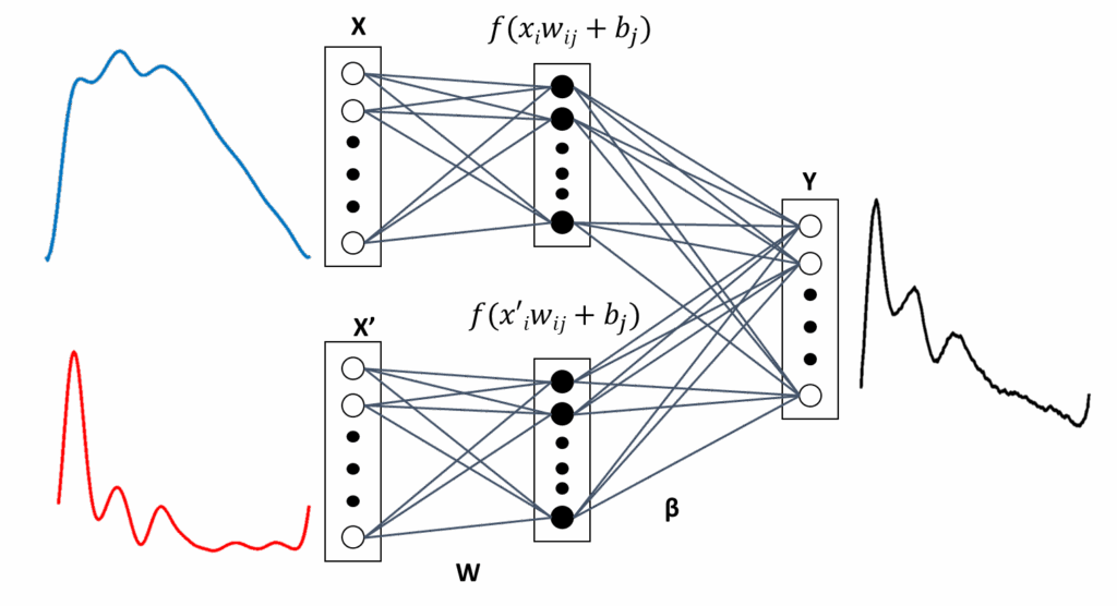
A third architecture ELM3, is used, which has a modular combination of PPG and VPG as input vector. As shown in Figure 6, ELM3 has two types of input vectors in separate modules and, because the hidden layer is not fully connected to all input neurons, they allow a different influence of PPG and VPG in fiAP or reBP estimation. In both cases, all of the neurons of the hidden layer are fully connected with all of the output neurons. ELM3’s output is represented in (12):

$$y_k \; g\left( \left[ \sum_{j1}^{M} f\left( \sum_{i1}^{N} w_{ji} x_i + b_j \right) \beta_{kj} + \sum_{lM1}^{2M} f\left( \sum_{i1}^{N} w_{li} x’_i + b_l \right) \beta_{kl} \right] \right) \tag{12}$$

where g and f are the same activation functions of the previous case and X  x₁, x₂, …, x_N is the sampled PPG and X′ x′₁, x′₂, …, x′_N is the sampled VPG.

3.7.2. Approach 2: SBP and DBP Estimates

SBP and DBP values are used as targets to train ELM4, ELM5 and ELM6. They correspond to reBP signal extreme values. To build the ELM models, we have used an ensemble approach to combine the inputs of different signals [39, 40].

The input vectors are those used in BP waveform estimation; except for PTT and HR, which are added as a second input vector module in ELM4 and ELM5, and as a third input vector module in ELM6. The output vectors are represented in two neurons, which codify SBP and DBP values.

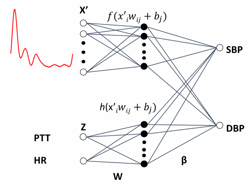
Figure 7 illustrates ELM4, which a modified architecture from ELM1. In addition to the sampled PPG waveform, a second module with the PTT and HR values is added. The same architecture is used with ELM5, which uses sampled VPG signals instead of those of the PPG. The ELM4 and ELM5 output vectors are obtained with (13):

$$y_k \; g\left( \sum_{j1}^{M} f\left( \sum_{i1}^{N} w_{ji} x_i + b_j \right) \beta_{kj} + \sum_{lM1}^{L} h\left( \sum_{i1}^{Q} w_{li} z_i + b_l \right) \beta_{kl} \right) \tag{13}$$

where the input signal X is the sampled PPG for the ELM4, and the sampled VPG for the ELM5. The input Z consists of two neurons for the PTT and HR values as input. Finally, f and h are linear activation functions.

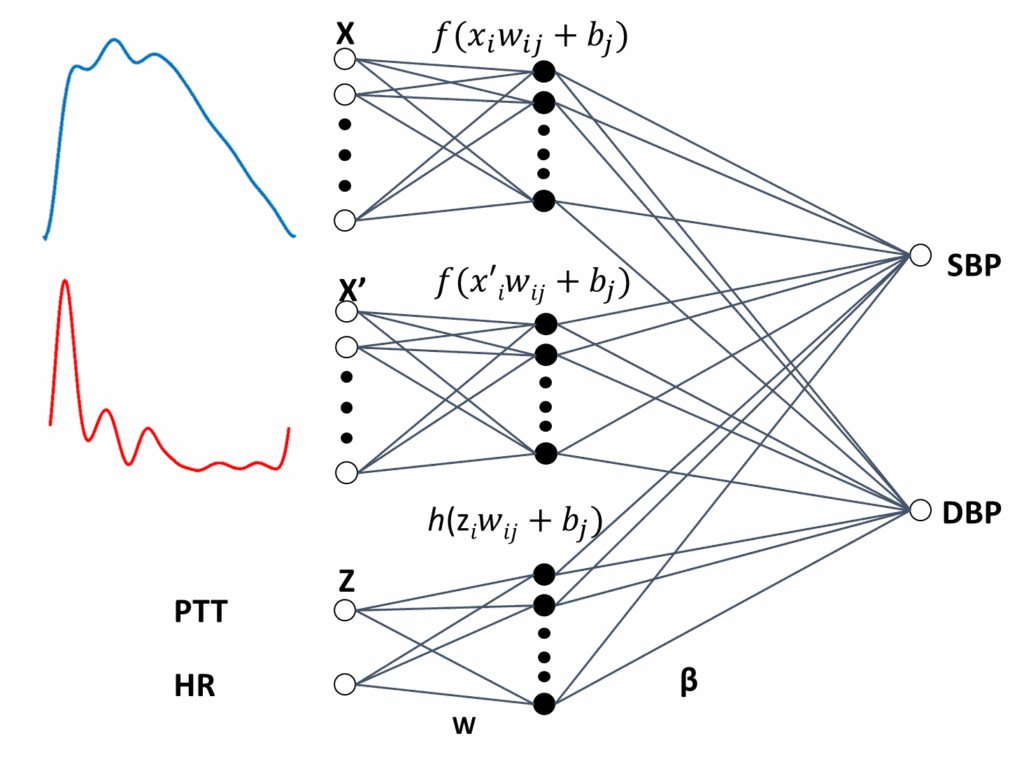
Finally, ELM6, which is the last architecture used, is illustrated in Figure 8. In this case, a modular combination of PPG with VPG, together with a third module for PTT and HR, are input vectors. The output vector is obtained in (14):

$$y_k \; g\left( \sum_{j1}^{M} f\left( \sum_{i1}^{N} w_{ji} x_i + b_j \right) \beta_{kj} + \sum_{pM1}^{P} f\left( \sum_{i1}^{N} w_{pi} x’_i + b_p \right) \beta_{kp} + \sum_{l2M1}^{L} h\left( \sum_{i1}^{Q} w_{li} z_i + b_l \right) \beta_{kl} \right) \tag{14}$$

where P 2M, X represents the PPG, X^′, is the VPG and Z correspond to input neurons for PTT and HR.

3.8. Hidden Layer Dimensionality

We use six different architectures of ELM to estimate BP in each subject. Our aim is to compare the capacity of ELM to estimate fiAP and reBP waveforms either from the PPG and VPG signals, and their combination, or to estimate SBP and DBP from the same signals. Nevertheless, a common problem in the design of the architecture of the multilayer perceptron is how to determine the number of neuron in the hidden layer [41]. This issue is considered in this pa- per by varying the number of neurons in the hidden layer for each of the ELM architectures and the performance for each architecture was tested. The dimension of the layer producing the smaller error for the test set is selected.

This procedure is especially powerful because one of the main advantages of ELM is its short training times. This characteristic allows us to perform exploratory studies to determine the suitable number of neurons to be used in the hidden layer. Tests in the range of 1–200 neurons in the hidden layer were performed. These tests showed that the best performance is achieved in the range of 14–23 neurons. This range of neurons is used in this work to search for the best architecture for each subject.

Table 2: Number of signals per subject that were used to train and test the ELM models

4. Results

4.1. Training and Testing Sets

Table 2 shows the number of heartbeats that are used to train and test ELM algorithms per subject. Each number is the result of signal processing and artifacts extractio–n from ECG, reBP, fiAP and PPG.

4.2. Fitting the fiAP Waveform

The LCD performance is shown in the last column of Table 3. These results are an extension of those in [22]. The main difference with the previous work is that only 160 heartbeats of 4 subjects are considered to fit PPG to the corresponding fiAP in that case, whereas in the current work PPG is fitted to fiAP during 4997 heartbeats of 15 subjects, which are taken from signals in the testing A mean relative error of 5.7 ± 1.6 with a mean r 0.95 are achieved for the 15 subjects.

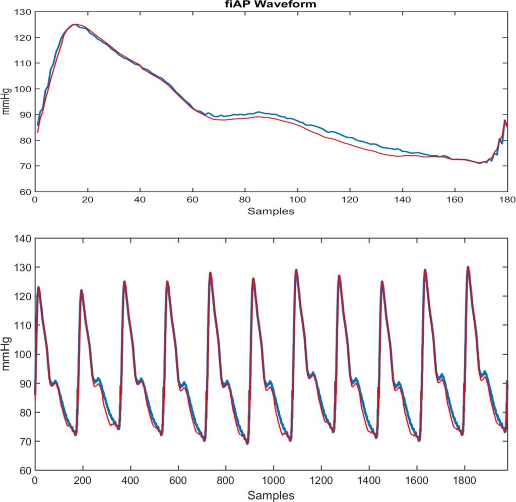
4.3. Estimating the fiAP Waveform

The fiAP waveform (in blue) and the ELM3 estimated wave- form (in red) is shown in the upper part of Figure 9. A strong similarity between them can be observed, with error < 5%. At the bottom of the figure, a train of fiAP waveforms (in blue) is shown with the ELM estimation (in red) above it. The estimation of the waveforms within the observed period is performed independently, beat to beat, and is then concatenated to form the train of BP pulses.

Table 3: Relative Error, its standard deviation (σ) and the correlation (r) from fiAP waveform estimation by ELMs with three types of training set: PPG waveform (ELM1); VPG waveform (ELM2) and a combination of PPG and VPG (ELM3). Finally a comparison with LCD fitting methodology

fiAP Waveform Estimate

Table 3 shows the relative error, with its standard devia- tion, and the correlation between measured fiAP waveform and ELM estimates for the 15 subjects. After applying the statistical t-test with a resulting p-value bigger than 0.05, we cannot conclude that a significant difference of the relative error exists between the ELM1, ELM2, ELM3 and LCD mod- els. However, with our data, the ELM models obtained the lowest mean relative error compared to the LCD. Moreover, there is no statistical significant difference in the correlations between the waveforms achieved by the models. The ELM models reach a correlation higher than 0.93 with an average of 0.97 ± 0.01.

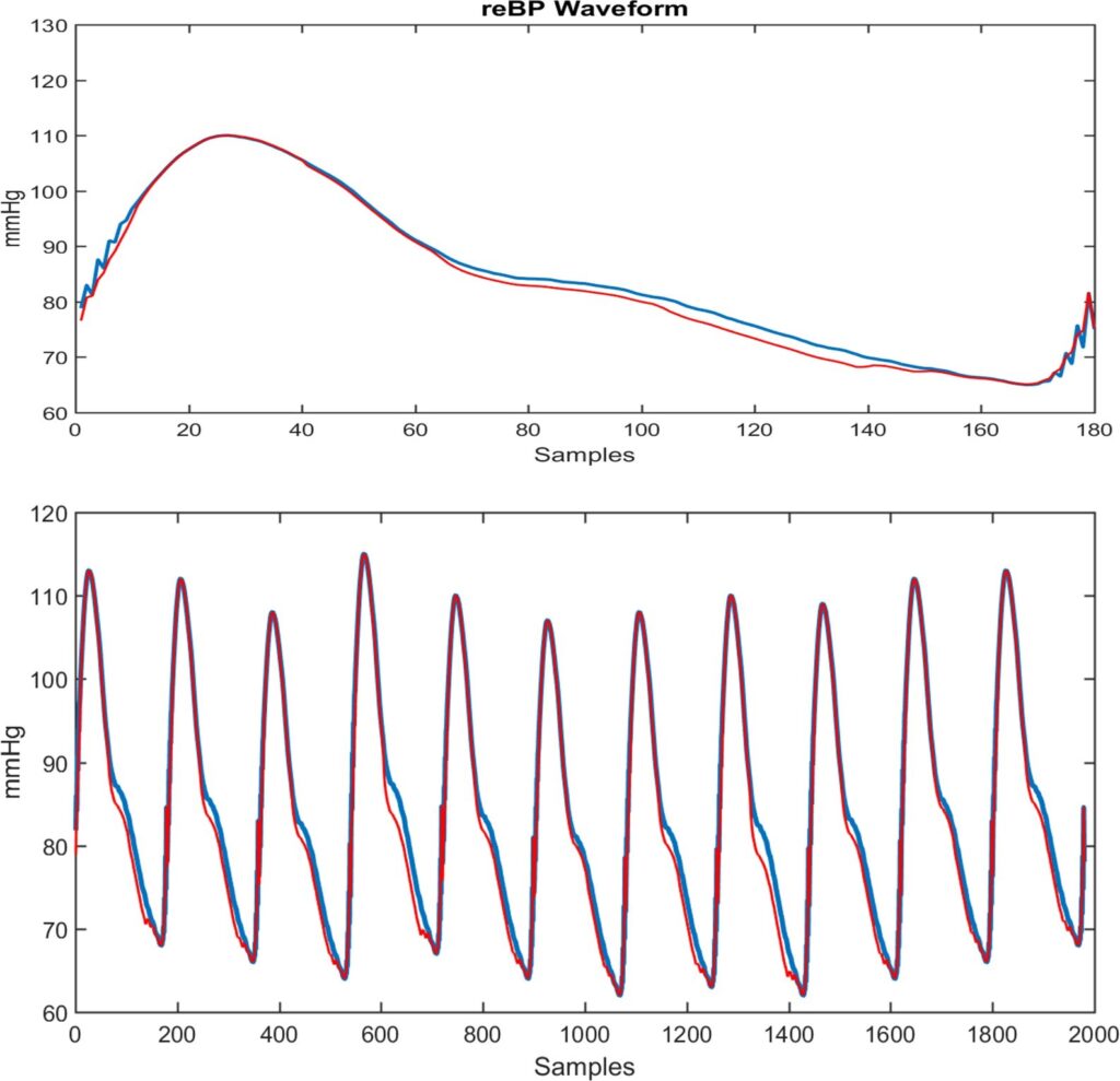
4.4. Estimating the reBP Waveform

Figure 10 shows at the top a reBP waveform (in blue) and the estimated waveform (in red) from the ELM with archi- tecture of Figure 6. A strong similarity can be seen. A train of reBP waveforms is shown at the bottom of Figure 10, with the ELM estimation above it. The estimation of each waveform is performed independently, beat to beat, and then concatenated to form the train of BP pulses.

Table 4 shows the relative error, with its standard devia- tion, and correlation between measured reBP waveform and ELMs estimates for the 15 subjects. The best result is slightly achieved by ELM3 (combination of PPG and VPG). After applying the statistical t-test with a resulting p-value bigger than 0.05, we cannot conclude that a significant difference of the relative error exists between the ELM1, ELM2, and ELM3 models. However, with our data, the ELM3, that combines PPG and VPG, obtained the lowest mean relative error of 3.33%. The ELM models reach a correlation higher than 0.96 with an average of 0.98 ± 0.01.

4.5. Estimating SBP

Table 5 shows the results of estimating SBP. After applying the statistical t-test with a resulting p-value bigger than 0.05, we cannot conclude that a significant difference of the relative error exists between the ELM4, ELM5, and ELM6 models. However, with our data, the ELM6 achieves the lowest mean relative error of 5.01% and the lowest average of the Root Mean Square Error of 5.86 mmHg. The minimum error is achieved for subject S 04 in all ELMs, having in ELM6 a RMSE: 2.6 mmHg and a relative error: 2.0%. The worse result is obtained in subject S 16 in all ELMs, having in ELM6 a RMSE: 12.6 mmHg and relative error: 13.5%.

Table 4: Relative Error, its standard deviation (σ) and the correlation (r) from reBP waveform estimation by ELMs with three types of training set: PPG waveform (ELM1); VPG waveform (ELM2) and a combination of PPG and VPG (ELM3)

reBP Waveform Estimate

Table 5: Root Mean Square Error (RMSE) and relative error from systolic BP estimation by ELMs with three types of training set: PPG waveform (ELM4); VPG waveform (ELM5) and a combination of PPG and VPG (ELM6). All of them plus PTT and HR correspond to each waveform

Systolic Blood Pressure Estimate

4.6. Estimating DBP

Table 6 shows the results of estimating DBP. After applying the statistical t-test with a resulting p-value bigger than 0.05, we cannot conclude that a significant difference of the relative error exists between the ELM4, ELM5, and ELM6 models. However, with our data, the ELM6 achieves the lowest mean relative error of 7.04% and the lowest average of the Root Mean Square Error of 4.78 mmHg.

The minimum error is achieved for subject S 04 in all ELMs, having in ELM6 a RMSE: 2.3 mmHg and relative error: 2.7%. The worse result is achieved in subject S 016 in all ELMs, having in ELM6 a RMSE: 9.3 mmHg and relative error: 19.1%.

Table 6: RMSE and relative error from diastolic BP estimation by ELMs with three types of training set: PPG waveform (ELM4); VPG waveform (ELM5) and a combination of PPG and VPG (ELM6). All of them plus PTT and HR correspond to each waveform

Diastolic Blood Pressure Estimate

5. Discussion

This work was inspired by a previous work [22], where in the LCD fitting process, 4997 signals are evaluated instead of the 160 signals per subject and the results are still surprising. They show a mean relative error RE 5.7 ± 1.6% and mean correlation r 0.95. These results allow us to assume that LCD really works and that derivative approaches are a suitable tool to fit the PPG waveform into the fiAP waveform.

However the ELM methods outperforms the performance of the LCD fitting process, where the ELM models reach a correlation higher than 0.96 with an average of 0.98 ± 0.01. Moreover, the ELM3 that consists in a modular combination of the PPG and VPG input signals, obtained the lowest mean relative error of 3.33%. Nevertheless, PPG and VPG were tested as inputs without being separated in two modules and the results were no better than PPG or VPG as independent inputs (ELM1 and ELM2).

Considering that PPG is measured with the index finger tip, it is surprising that ELM has better results estimating the reconstructed brachial BP waveform than fiAP wave- form. The fiAp is measured in the digital artery of the middle finger, next to the finger where PPG is measured. Consequently, it is expected that fiAP waveform estimates should be better than reBP waveform estimates because digital artery is a distal branch of the brachial artery and, therefore, it could be assumed that it is more complex to estimate reBP waveform than fiAP waveform.

In [23] – [25], the authors have evaluated the performance of the Deep Boltzmann machine and Support Vector Regressions as machine learning models used to estimate the Blood Pressure. These models were tested with BP and PPG waveforms of subjects whose datasets were randomly combined and separated in training and test sets afterwards (Similar signals appears in training and test sets). Moreover, they have not induced a blood pressure rise. Under this scenario, the models show a good performance. On the other hand, our proposed model is able to estimate high pressure data obtained by induced handgrip maneuver, this data is a realistic simulation of high pressure events. Our results shows an acceptable mean relative error.

Improving the results in SBP, DBP and waveform estimations may help to start the development of a new technique in BP estimation, which combines two very important aspects in BP studies: its extreme values and its waveform (See [42] for naming standards of these features).

In addition, in a preliminary way, several tests were carried out with inter-subject data and ELM obtained poor results when the subjects have very different biometric characteristics. However, with two similar subjects, good estimates were obtained, which are: healthy male subjects, aging 26 and 27 years old, and Body Mass Index close to 22.5 [Kg / m2]. In this case, ELM achieved SBP and DBP values estimates with errors less than 10%. This suggests that, as expected, more data needs to be collected to achieve the different existing clusters, each of which with sufficient data size. This may allow the demands for completeness and consistency of the training and testing data to be satisfied. Therefore, following the theorem applicable to single inter- mediate layer artificial neural networks that can perform as universal Approximators [43], the achievement of nImI methods to estimate BP from PPG is granted for all subjects belonging to any cluster.

This research provides the following contributions and improvements:

• The main goal was to develop a machine learning method to estimate the arterial blood pressure from PPG and VPG signals measured from healthy subjects.
• We have validated the Extreme Learning Machine (ELM) as a model that relates the PPG to fiAP and brachial reconstructed Blood Pressure (reBP) wave- forms.

• We have validated the Extreme Learning Machine as a model used to estimate the Systolic and Diastolic BP values.
• We have evaluated how a combination of PPG and its derivatives can improve the performance compared to using only the signal by itself.
• We have evaluated how the incorporation of signif- icant parameters extracted from the original signal such as PTT and HR can enhance the performance of the ELM.
• We have conducted a clinical essay approved by the Bioethics Institutional Committee for Human Beings Research of the Universidad de Valparaiso. In the procedure, the volunteers performed two handgrips, which is isometric maneuver to induce controlled Blood Pressure rises.

6. Conclusions

In this work, ELM is conclusively shown to be a suitable tool to estimate BP from PPG when input vectors are PPG related data, and target vectors, either, fiAP and reBP waveforms, or, SBP and DBP values that belong to the same subject.

These are promising results and they suggest that we should continue our research into machine learning and its potential in health applications. ELM has good results estimating the brachial BP waveform and other main arteries can perhaps be studied with this type of architecture and method, such as the aorta, which a very important artery in cardiovascular studies.

Although both SBP and DBP estimations show promis- ing results, they still need to be more precise because a maximum error of ±3 mmHg is accepted for BP medical devices. Nevertheless, different architectures and inputs from PPG, and its derivative approaches, can be evaluated to help the ELM learning process.

We have also tested the inter-subject Blood pressure estimation, however more work and research are required to enhance the performance. We think that if the number of subjects recruited is increased considerable, then there will be a chance to have a global model instead of a individual ad-hoc subject model.

Future work is required in order to increase the number of subjects and thus increase the variability of the signals. Furthermore, it would be interesting to explore other methods such as neuro-fuzzy models [40, 44], machine learning models [45], and deep learning techniques [46]. Moreover, analysing the wavelet domain of the signals could be relevant for healthcare applications [47, 48]. On the other hand, information from experts could be included in the models [49] and potential biomarkers could be found using machine learning techniques [50].

Conflict of Interest The authors declare no conflict of interest.

Acknowledgments

The authors acknowledge the support given by Chilean ANID Grants FONDEF IT13I20060, Fondo Nacional de Desarrollo Científico y Tecnológico Fondecyt Nº 1221938, PAI Folio 79140057, CIDIS-UV 14 and ANID – Millennium Science Initiative Program ICN2021-004.

The authors also acknowledge to anonymous healthy volunteers who participate in the clinical essays that were approved by the Interdisciplinary Bioethics Research Com- mittee in Human Beings (CIBI- SH), of Valparaíso University (Chile)

1. R. Victor, Hipertensión arterial sistémica: mecanismos y diagnóstico, vol. 1, chap. 45, pp. 944–963, Elsevier, Barcelona, 9th ed., 2013.
2. S. A. Esper, M. R. Pinsky, “Arterial waveform analysis”, Best Practice & Research Clinical Anaesthesiology, vol. 28, no. 4, pp. 363–380, 2014, doi:10.1016/j.bpa.2014.08.002.
3. N. Kaplan, Hipertensión arterial sistémica: mecanismos y diagnóstico, in Braunwald (Ed) Tratado de cardiología, Madrid: Marbán Libros.Edition 6., 2004.
4. I. Moxham, “Understanding arterial pressure waveforms”, Southern African Journal of Anaesthesia and Analgesia, vol. 9, no. 1, pp. 40–42, 2003.
5. F. Mahomed, “The physiology and clinical use of the sphygmograph”,
   Med Times Gazette, vol. 1, p. 507, 1872.
6. S. W. Moss, Edgar Holden, MD of Newark, New Jersey: Provincial Physician on a National Stage, Xlibris Corporation, 2014.
7. M. F. O’Rourke, A. Pauca, X.-J. Jiang, “Pulse wave analysis”, British journal of clinical pharmacology, vol. 51, no. 6, pp. 507–522, 2001, doi: 10.1046/j.0306-5251.2001.01400.x.
8. I. B. Wilkinson, H. MacCallum, L. Flint, J. R. Cockcroft, D. E. Newby,
   D. J. Webb, “The influence of heart rate on augmentation index and central arterial pressure in humans”, The Journal of physiology, vol. 525, no. 1, pp. 263–270, 2000.
9. M. F. O’Rourke, D. E. Gallagher, “Pulse wave analysis”, Journal of Hypertension-Supplement-, vol. 14, pp. S147–S158, 1996.
10. R. A. Payne, I. B. Wilkinson, D. J. Webb, “Arterial stiffness and hy- pertension emerging concepts”, Hypertension, vol. 55, no. 1, pp. 9–14, 2010, doi:10.1161/HYPERTENSIONAHA.107.090464.
11. R. R. Townsend, H. R. Black, J. A. Chirinos, P. U. Feig, K. C. Ferdinand,
    M. Germain, C. Rosendorff, S. P. Steigerwalt, J. A. Stepanek, “Clinical use of pulse wave analysis: Proceedings from a symposium sponsored by north american artery”, The Journal of Clinical Hypertension, vol. 17, no. 7, pp. 503–513, 2015, doi:10.1111/jch.12574.
12. J. Peňaz, “Photoelectric measurement of blood pressure, volume and flow in the finger”, “Digest of 10th International Conference on Medical Biological Engineering, Dresden, East Germany”, p. 104, 1973.
13. N. Westerhof, M. F. O’Rourke, “Haemodynamic basis for the devel- opment of left ventricular failure in systolic hypertension and for its logical therapy.”, Journal of hypertension, vol. 13, no. 9, pp. 943–952, 1995.
14. K. S. Matthys, A. F. Kalmar, M. M. Struys, E. P. Mortier, A. P. Avolio, P. Segers, P. R. Verdonck, “Long-term pressure monitoring with arte- rial applanation tonometry: a non-invasive alternative during clinical ervention?”, Technology and Health Care, vol. 16, no. 3, pp. 183–193,008.
15. R. Payne, C. Symeonides, D. Webb, S. Maxwell, “Pulse transit time measured from the ecg: an unreliable marker of beat-to-beat blood pressure”, Journal of Applied Physiology, vol. 100, no. 1, pp. 136–141, 2006.
16. J. Allen, “Photoplethysmography and its application in clinical physi- ological measurement”, Physiological measurement, vol. 28, no. 3, pp. R1–R39, 2007, doi:10.1088/0967-3334/28/3/R01.
17. D. Zheng, J. Allen, A. Murray, “Determination of aortic valve opening time and left ventricular peak filling rate from the peripheral pulse amplitude in patients with ectopic beats”, Physiological measurement, vol. 29, no. 12, p. 1411, 2008.
18. R. Lazazzera, Y. Belhaj, G. Carrault, “A new wearable device for blood pressure estimation using pthotoplethysmogram”, Sensors, vol. 19, no. 2557, p. s19112557, 2019, doi:10.3390/s19112557.
19. Y. Chen, L. Li, C. Hershler, R. P. Dill, “Continuous non-invasive blood pressure monitoring method and apparatus”, 2003, uS Patent 6,599,251.
20. M. Y.-M. Wong, C. C.-Y. Poon, Y.-T. Zhang, “An evaluation of the cuffless blood pressure estimation based on pulse transit time tech- nique: a half year study on normotensive subjects”, Cardiovascular Engineering, vol. 9, no. 1, pp. 32–38, 2009.
21. G. Tapia, A. Glaría, “Artificial neural network detects physical stress from arterial pulse wave”, Revista Ingeniería Biomédica, vol. 9, no. 17, pp. 21–34, 2015.
22. G. Tapia, M. Salinas, J. Plaza, D. Mellado, C. Saavedra, Veloz, A. Ar- riola, R. Salas, A. Glaría, “Photoplethysmogram fits finger blood pressure waveform for non-invasive and minimally-intrusive technologies”, “Biosignal: 10th International Joint Conference on Biomed- ical Engineering Systems and Technologies. Biostec 2017”, vol. 4, pp. 155–162, Porto, 2017.
23. M. W. K. Fong, E. Ng, K. E. Z. Jian, T. J. Hong, “SVR ensemble- based continuous blood pressure prediction using multi-channel photoplethysmogram”, Computers in Biology and Medicine, vol. 113, p. 103392, 2019, doi:10.1016/j.compbiomed.2019.103392.
24. S. Chen, Z. Ji, H. Wu, Y. A. Xu, “A non-invasive continuous blood pressure estimation approach based on machine learning”, Sensors, vol. 2585, p. 19, 2019, doi:10.3390/s19112585.
25. S. Lee, J.-H. Chang, “Dempster–shafer fusion based on a deep boltz- mann machine for blood pressure estimation”, Applied Science, vol. 96, p. 9, 2019, doi:10.3390/app9010096.
26. G. Huang, G.-B. Huang, S. Song, K. You, “Trends in extreme learn- ing machines: a review”, Neural Networks, vol. 61, pp. 32–48, 2015, doi:10.1016/j.neunet.2014.10.001.
27. H. Allende, C. Moraga, R. Salas, “Artificial neural networks in time series forecasting: A comparative analysis”, Kybernetika, vol. 38, no. 6, pp. 685–707, 2002.
28. D. E. Rumelhart, G. E. Hinton, R. J. Williams, “Learning representa- tions by back-propagating errors”, Cognitive modeling, vol. 5, no. 3, p. 1, 1988.
29. G.-B. Huang, Q.-Y. Zhu, C.-K. Siew, “Extreme learning machine: the- ory and applications”, Neurocomputing, vol. 70, no. 1, pp. 489–501, 2006, doi:10.1016/j.neucom.2005.12.126.
30. E. Cambria, G.-B. Huang, L. L. C. Kasun, H. Zhou, C. M. Vong, J. Lin,
    J. Yin, Z. Cai, Q. Liu, K. Li, et al., “Extreme learning machines [trends & controversies]”, IEEE Intelligent Systems, vol. 28, no. 6, pp. 30–59, 2013, doi:10.1109/MIS.2013.140.
31. G.-B. Huang, Q.-Y. Zhu, C.-K. Siew, “Extreme learning machine: a new learning scheme of feedforward neural networks”, “Neural Net- works, 2004. Proceedings. 2004 IEEE International Joint Conference on”, vol. 2, pp. 985–990, IEEE, 2004, doi:10.1109/IJCNN.2004.1380068.
32. G. Tapia, J. Plaza, M. Salinas, A. Glaria, “Training set for nimi blood pressure estimates v 1.0 minimally documented training set nimi data
    1.0 documentation”, http://nimi.uv.cl, 2017.
33. Finapres, “Finapres medical systems (2015)”, http://www.finapres. com/products/finapres-nova, 2015, accessed: 2015-04-18.
34. J. Pan, W. J. Tompkins, “A real-time QRS detection algorithm”, IEEE transactions on biomedical engineering, vol. 32, no. 3, pp. 230–236, 1985.
35. A. C. Guyton, J. E. Hall, Tratado de fisiología médica, Elsevier„ Barcelona, 12 ed., 2011.
36. M. Elgendi, “Standard terminologies for photoplethysmogram sig- nals”, Current cardiology reviews, vol. 8, no. 3, pp. 215–219, 2012, doi:10.2174/157340312803217184.
37. E. Zahedi, K. Chellappan, M. A. M. Ali, H. Singh, “Analysis of the effect of ageing on rising edge characteristics of the photoplethysmo- gram using a modified windkessel model”, Cardiovascular Engineering, vol. 7, no. 4, pp. 172–181, 2007.
38. M. Salinas, R. Salas, D. Mellado, A. Glaría, C. Saavedra, “A computa- tional fractional signal derivative method”, Modelling and Simulation in Engineering, vol. 2018, p. 7280306, 2018, doi:10.1155/2018/7280306.
39. H. Allende, C. Moraga, R. Ñanculef, R. Salas, “Ensembles methods for machine learning pattern recognition and machine vision”, Series Information Sciences & Tecnology. In honor and memory of Prof. KS. Fu, pp. 247–261, 2010.
40. M. Querales, R. Salas, Y. Morales, H. Allende-Cid, H. Rosas, “A stacking neuro-fuzzy framework to forecast runoff from distributed meteorological stations”, Applied Soft Computing, vol. 118, p. 108535, 2022, doi:10.1016/j.asoc.2022.108535.
41. G. Feng, G.-B. Huang, Q. Lin, R. Gay, “Error minimized extreme learning machine with growth of hidden nodes and incremental learning”, IEEE Transactions on Neural Networks, vol. 20, no. 8, pp. 1352–1357, 2009, doi:10.1109/TNN.2009.2024147.
42. M. Elgendi, Y. Liang, R. Ward, “Toward generating more diagnostic features from photoplethysmogram waveforms”, Diseases, vol. 20, p. 6, 2018, doi:10.3390/diseases6010020.
43. K. Hornik, M. Stinchcombe, H. White, “Multilayer feedforward net- works are universal approximators”, Neural networks, vol. 2, no. 5, pp. 359–366, 1989.
44. Y. Morales, M. Querales, H. Rosas, H. Allende-Cid, R. Salas, “A self-identification neuro-fuzzy inference framework for modeling rainfall-runoff in a chilean watershed”, Journal of Hydrology, vol. 594, p. 125910, 2021, doi:10.1016/j.jhydrol.2020.125910.
45. A. Bertini, R. Salas, S. Chabert, L. Sobrevia, F. Pardo, “Using ma- chine learning to predict complications in pregnancy: A systematic review”, Frontiers in bioengineering and biotechnology, vol. 9, 2021, doi:10.3389/fbioe.2021.780389.
46. D. Mellado, C. Saavedra, S. Chabert, R. Torres, R. Salas, “Self- improving generative artificial neural network for pseudorehearsal incremental class learning”, Algorithms, vol. 12, no. 10, p. 206, 2019, doi:10.3390/a12100206.
47. C. Saavedra, R. Salas, L. Bougrain, “Wavelet-based semblance meth- ods to enhance the single-trial detection of event-related potentials for a bci spelling system”, Computational Intelligence and Neuroscience, vol. 2019, 2019, doi:10.1155/2019/8432953.
48. E. Vivas, H. Allende-Cid, R. Salas, L. Bravo, “Polynomial and wavelet- type transfer function models to improve fisheries’ landing forecasting with exogenous variables”, Entropy, vol. 21, no. 11, p. 1082, 2019, doi: 10.3390/e21111082.
49. E. Cantor, R. Salas, H. Rosas, S. Guauque-Olarte, “Biological knowledge-slanted random forest approach for the classification of calcified aortic valve stenosis”, BioData Mining, vol. 14, no. 1, pp. 1–11, 2021, doi:10.1186/s13040-021-00269-4.
50. P. Franco, J. Sotelo, A. Guala, L. Dux-Santoy, A. Evangelista,J. Rodríguez-Palomares, D. Mery, R. Salas, S. Uribe, “Identification of hemodynamic biomarkers for bicuspid aortic valve induced aortic in biology and medicine, 10.1016/j.compbiomed.2021.105147.

Citations by Dimensions

Citations by PlumX

Crossref Citations

This paper is currently not cited.

No. of Downloads per Month

No. of Downloads per Country