VSC-HVDC Robust LMI Optimization Approaches to Improve Small-Signal and Transient Stability of Highly Interconnected AC grids

(This article belongs to the Section Automation and Control Systems (ACS))
Export Citations
Cite
Xing, Y. , Kamal, E. , Marinescu, B. and Xavier, F. (2022). VSC-HVDC Robust LMI Optimization Approaches to Improve Small-Signal and Transient Stability of Highly Interconnected AC grids. Journal of Engineering Research and Sciences, 1(5), 251–263. https://doi.org/10.55708/js0105026
Yankai Xing, Elkhatib Kamal, Bogdan Marinescu and Florent Xavier. "VSC-HVDC Robust LMI Optimization Approaches to Improve Small-Signal and Transient Stability of Highly Interconnected AC grids." Journal of Engineering Research and Sciences 1, no. 5 (May 2022): 251–263. https://doi.org/10.55708/js0105026
Y. Xing, E. Kamal, B. Marinescu and F. Xavier, "VSC-HVDC Robust LMI Optimization Approaches to Improve Small-Signal and Transient Stability of Highly Interconnected AC grids," Journal of Engineering Research and Sciences, vol. 1, no. 5, pp. 251–263, May. 2022, doi: 10.55708/js0105026.
In this paper, for the situation of HVDC inserted in meshed AC power grid, a model-matching robust H∞ static output error feedback controller (RSOFC) and model-matching dynamic decoupled output feedback controller (DDOFC) are proposed to improve the damping of inter-area oscillation modes and maintain robustness to face the effects of different operating points and unstable zeros. Sufficient conditions for robust stability are derived in the sense of Lyapunov asymptotic stability and presented in the form of linear matrix inequalities to obtain H∞ RSOFC and DDOFC gains based on the reference model. The efficiency and robustness of the proposed controllers are tested and compared to Linear-Quadratic-Gaussian (LQG) control, mixed sensitivity H∞, standard (IEEE) Power Oscillation Damping (POD) controllers on a realistic benchmark of 19 generators connected by a meshed AC grid. The main contributions of this paper are: (i) Compensate the negative effect of unstable zeros (non-minimum phase behavior) on the performances of the closed-loop; (ii) the robustness is improved in order to provide good responses in case of network variations (load evolution, line, and generator trips, etc.) and HVDC line parameters changes; (iii) improve the damping compared with standard controller structures (LQG, mixed sensitivity H∞ and standard POD controller).
1. Introduction
The traditional electricity transmission system based on three-phase AC grids, in general, works well and with good levels of reliability. However, there are challenges arising mainly from environmental impact and the increase in the renewable generation, (according to [1] the next decade will be devoted to the large-scale exploitation of offshore wind energy, which means the need to transport electrical energy over long distances to establish a connection with the main power grid). This will likely increase the level of variability and unpredictability in the operation of power grids, leading to an increased need for power reserves for balancing energy consumption and will require more flexible power flow control. The solution that overcomes these problems is the use of high voltage direct current (HVDC) transmission systems, which are more feasible and also more competitive than traditional transmission systems (HVAC), especially with the development of power electronics components. One of the most important advantages of this technology against the HVAC technology is that the former is suitable for long distances with minimal losses. The second advantage is the right-of-way; it is often easier to get permission for underground DC cables due to the reduced environmental impact [2]. The HVDC system is a power electronics technology used in electrical power systems primarily because of ability to transmit large amounts of energy over long distances [3]. In the case of HVAC systems the power transfer is limited because of the difference between the voltage angles of the terminals which increases with distance [4]. To solve this problem the network operator can use reactive power means of reactive power compensation along the line, such as such as FACTS (Flexible Alternating Current Transmission System) devices. However, these devices are very expensive and cannot always be installed in the most appropriate place. Once the development of high power switching devices and their devices and their availability at low prices, Line-commutated converters (LCCs) which used thyristors as the basic as a basic component in HVDC were replaced by voltage source converters (VSCs) [3]. Since VSC- HVDC has been gradually incorporated into the grid, they can be utilized to suppress low-frequency oscillations. The modes usually considered in the past were the most spread inter-area ones which are at low frequencies (in Europe about 0.2 Hz). For HVDC inserted in a meshed AC network, such as the recent interconnection reinforcements in Europe, inter-area modes corresponding to a limited number of generators in the area near the HVDC may be involved. They are at a higher frequency, around 1 Hz. However, in this frequency range, inter-area modes are close to other modes of a different nature (see [5, 6]) which are disturbed by the HVDC power oscillation damping (POD) controller. The use of classical Institute of Electrical and Electronics Engineers (IEEE) POD controller structures and tuning methods (see e.g. [7]) are focused on only one mode, and tends to inefficient damping and destabilize other modes.
It is well known that unstable zeros can degrade the performance of the control system. However, there is rare research on the origin of unstable zeros in HVDC links inserted into meshed AC networks. Therefore, it is important in research and practice to analyze network parameters with HVDC links to highlight their influence on unstable zeros. In addition, modeling errors and system uncertain- ties in plant models are inevitable in many applications. To ensure accuracy, design techniques must take these errors and uncertainties into account to be practical. Therefore, a (robust) control approach must be used to deal with the uncertainties arising from operating point changes in the power system, as well as the modeling errors caused by modeling and model reduction of realistic power systems.
Hence, the contributions of this paper, based on the afore- mentioned works are to develop robust POD controllers which improve the damping of aforementioned high frequency inter-area modes without deteriorating the damping of the others and to eliminate the impact of unstable zeros. To develop advanced control one usually needs a state-space representation of the system [8], [9]. In [10], it is studied in detail the stability at small perturbations with power stabilizers (PSSs) in order to satisfy some recent objectives and constraints imposed by the evolution of large-scale interconnected power systems. H∞ or H2 approaches in the field of robust control are studied in a huge number of publications since the mid-1980s. In the context of robust control of linear systems, modern multivariate synthesis methods integrate a model of the process with a family of systems. They use a deviation model, which is defined either by different types of norms in the frequency or time domain, or by uncertainty domains on the parameters, or by sectors of the complex plane. For some types of error modeling, a synthesis technique is associated. A presentation of these different techniques will be proposed, with particular attention to those based on the use of H and H2. The H optimal control is used to control a system subject to modeling errors and parametric uncertainties [11]. In [12], an H controller is compared to a controller obtained by a LQG/LTR (Loop Transfer Recovery) method, allowing to recover some robustness properties of the LQ (in the sense of modulus margin and not parametric ro- bustness). The H2 methodology was applied in [13], to find state feedback controller offering a satisfactory the required performance. The paper [14] proposes an iterative methodology in order to obtain a static output controller by a mixed H2/H synthesis. Many works deal with the analysis of stability and the stabilization to design robust dynamic output-feedback controllers [15], [16] based on Linear matrix inequalities (LMI). LMI are used to solve several problems of automation, (optimization problems in control theory, system identification,…) which are generally difficult to solve analytically. The interest of methods based on LMIs comes from the fact that they can be solved using convex programming [17]-[19]. With this approach, one is no longer limited to problems with an analytical solution. By solving these inequalities, one obtains a domain of feasible solutions, i.e. solutions satisfying these LMIs, larger than the one generated by the search for analytical solutions. Using the fact that an inequality has more solutions than an equation it is possible to use the additional degrees of freedom to include other objectives than those than those initially chosen. The notions of LMIs are found in several works since many years. Thus Lyapunov conditioned the stability of a system by LMI [20]. In the work presented here, two model-matching based methods are proposed to solve above mentioned problems. The contributions and novelty of this paper are: i) Firstly, the reference model in this work is proposed as having the desired characteristics, which means to horizontally shift the poles to left in the complex plane until getting the desired damping (over 10 %). Moreover, unstable zeros of the control model are shifted to left plane which is closed to the vertical axis to decrease the control difficulty. ii) Secondly, sufficient conditions are derived based on LMIs for robust stabilization, in the sense of Lyapunov method to obtain robust H static output error feedback controller (RSOFC) and dynamic decoupled output feedback controller (DDOFC) gains based on the reference model. iii) Thirdly, different controls from the literature (Linear-quadratic-Gaussian (LQG), mixed sensitivity H and standard (IEEE) Power Oscillation Damping (POD) controllers) are implemented for the realistic benchmark of 19 generators connected by a meshed AC grid to compare with the proposed H∞ RSOFC and DDOFC. The rest of the paper is organized as follows. Section 2 presents the problem statement and control model of the realistic benchmark of 19 generators connected by a meshed AC grid. The stability and the design of the proposed strategies are studied in Section 3. Section 4 introduces the proposed RSOFC and DDOFC. In Section 5, a simulation study to evaluate the performances of the proposed strategies is presented. In the Section 6 we present the conclusions and future works.
2. Problem Formulation, Main Difficulties and Modeling
2.1. Test system
A test system with aforementioned particularities is pro- posed. It contains an HVDC line inserted into an AC network consisting of 19 generators. All generators are controlled by AVR (Automatic Voltage Regulator) and PSS (Power System Stabilizer). The order of full nonlinear system is 724, which is linearized to obtain the full linear model of the same order. The less damped and highest residue modes found in Table 1 (see details in [21]).
2.2. Control model
In this paper the studied control model is developed in our previous work [21], [22]. By definition, a linear system is a system governed by ordinary linear differential (or even algebraic) equations with non-constant coefficients. They describe the temporal evolution of the constituent variables
Table 1: The linearized model
No. | Mode | Damping ξ (%) | Freq. (Hz) | Mode shape (participation mag (%)) Residue | |||
GE_91−3 (32.4) | ABS MAG | Phase | |||||
1 2 3 4 5 6 7 8 9 10 | -1.62+j8.19 -0.24+j5.53 -0.53+j5.29 -0.40+j4.79 -0.33+j3.29 -18.83+j7.21 -1.54+j6.55 -19.32+j6.47 -20.33+j4.86 -18.72+j3.35 | 19.5 4.5 10.1 8.3 10.1 93.3 22.9 94.8 97.2 98.4 | 1.30 0.88 0.84 0.76 0.52 1.14 1.04 1.03 0.77 0.53 | GE_914 (100) GE_911 (100) GE_917 (100) GE_918 (44.3) GE_915 (100) GE_921, GE_922 (100) GE_914 (100) GE_921 (100) GE_921, GE_922 (84.5) GE_913 (33.4) | GE_917 (68.8) GE_918 (55.1) GE_912 (100) GE_918 (17.7) GE_923, GE_924 (74.1) GE_911 (68.3) GE_922 (37.6) GE_927 (100) GE_912 (100) | 0.0157 0.0181 0.0129 0.0038 0.0121 0.0034 0.0125 0.0117 0.0026 0.0072 | 35.0 83.4 -56.2 -33.3 104.5 14.5 151.5 118.9 -168.1 136.1 |
(state variables) of the physical system. This broad definition explains the complexity, the diversity of linear systems as well as the variety of methods that apply to them. A state representation of a linear system is given by:
$$\begin{bmatrix} x \\ y \end{bmatrix} = \begin{bmatrix} A & B \\ C & 0 \end{bmatrix} \begin{bmatrix} x \\ u \end{bmatrix}
\tag{1}$$
where x ∈ ℜn×1 is the state vector of the system, y ∈ ℜg×1 is the measured output vector and u ∈ ℜm×1 is the input vector, C ∈ ℜg×n, A ∈ ℜn×n and B ∈ ℜn×m, are matrices of linear functions.
In our case, y ∆θ and u is Q , where Q is the reactive power, ∆θ θ1_ θ2 is the difference of angles of the terminal voltages [23].
2.3. Classic POD
The detailed classic POD in this paper is proposed based on [7], [21], [22]. It is defined by the transfer function given by (2). The classical adjustment of the parameters of this system is given in the [24]. For the desired damping of 10% set for mode 2 in Table 1, The classic POD tuning parameters K, T1, T2, Tw and n are defined in [22].
$$H_{PODS} = K \left( \frac{T_w s}{1 + T_w s} \right) \left( \frac{1 + T_1 s}{1 + T_2 s} \right)^n\tag{2}$$
2.4. Main objectives and difficulties
- Particular frequency range of inter-area modes: As mentioned in Introduction, in highly meshed AC grid, the inter-area modes are at higher frequency. In this range of frequency, other types of modes exist: local modes and electric coupling modes or general electric modes linked to other electric phenomena. In the theory of systems, the models used for the design of control laws are often models of reduced size. How- ever, the increase in electrical interconnections has caused the increase in the size of models representing these electrical systems. This makes their use for the design of controllers almost impossible. Moreover, the extension of the European synchronous area to the east of Europe has not only made the volume of numerical calculations in the field of “electrical” systems, but also changed the frequencies of the inter-area modes. These modes are associated with oscillations involv- ing a number of machines distant from the electrical system and will be defined in in detail in [5]. More precisely, these modes shift to lower frequencies (by about a decade), which makes the gap between the frequency of the inter-area modes and the local modes (which concern only one generator) which remain in high frequency ranges. This deviation considerably modifies the global transient behavior of the electrical system and makes it difficult to synthesize controllers for a mixed specification, i.e., for both inter-area and local modes. In the previous works, the regulator de- sign approaches use a simplified model consisting of a machine connected through a line of reactance X to the rest of the electrical system modeled by an infinite bus. Although this simplified model, also called “single machine on infinite bus”, is very small compared to the full model of the electrical system, it cannot repro- duce the dynamic phenomena concerning the voltage regulation specifications in the case of the very large systems mentioned above. Indeed, this model has only one inter-area mode which frequency depends on the parameter X, i.e., the length of the line connect- ing the machine to the infinite bus. It cannot therefore reproduce both local and inter-area local modes and inter- area modes of much lower frequency. Therefore, controllers designed with this model are not very efficient to meet the above-mentioned requirements. In [25], the balanced realization of an electrical system (representation of a complete electrical system by a reduced system containing only the most controllable and observable oscillatory modes) has been used for the construction of a control model allowing an opti- mal choice of the PSS locations to prevent blackouts in electrical systems. Although the chosen locations of the controls and measures improve the stability of the electrical system in the general case, these models are not optimal from the point of view of the most controllable and observable modes are not the un- damped modes of the system. To answer this problem, we have proposed in this paper to use the control model built from the complete model representing the electrical system. This model allows, by preserving an important set of variables and oscillatory modes of the complete model, to reproduce a given oscillatory behavior of the complete system which has both local and global components, i.e., that involves both local and global modes. Therefore, the controllers designed with this model will have an effective action once implemented in the complete system.
- Unstable zeros: The existence of unstable zeros in the HVDC embedded system depends on the topology of the grids [26]. The effectiveness of POD can be decreased because of these unstable zeros [27].
- Uncertainty of system: The modeling of a physical system is a crucial phase in the synthesis of the Due to uncertainties, the mathematical model may not reflect the physical reality of the system. Nevertheless, if we manage to characterize these uncertainties, it is possible to complete the nominal model with an additional uncertain part. The sources of uncertainties are numerous but they are generally classified in two categories.
- Non-structural uncertainties also called non- parametric. They represent external dynamics, for example: measurement noise, external disturbances, etc. disturbances, etc. In general, their dynamics are unknown and we have no information on the way they act on the system. On the other hand, we know that they are bounded in norms.
- Structural uncertainties also called modeling or parametric They are generally due to approximation errors and/or simplifications necessary to obtain an exploitable control model reflecting the real dynamics of the physical system.
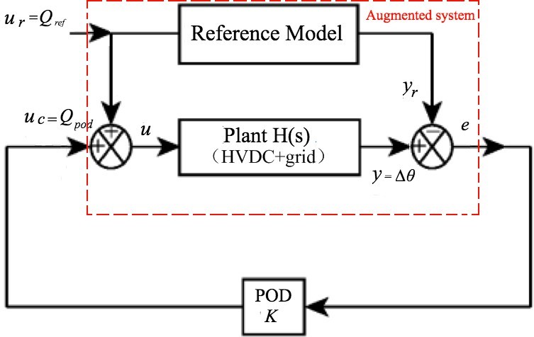
In this paper, we design the controller for control model (1) (cf. Fig. 1) subject to the non-structural uncertainties.
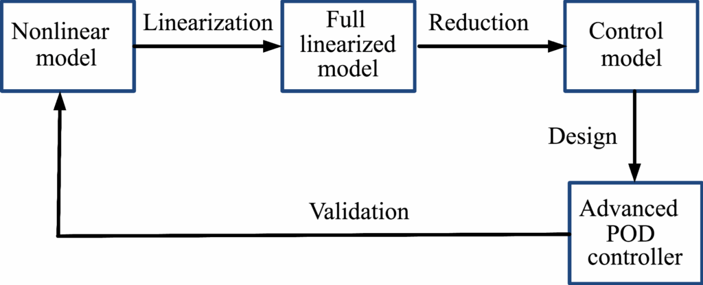
It should be noted that all these requirements cannot be fully satisfied neither with the classic POD recalled in Section 2.3, nor with the standard H2 and H∞ robust controllers. To overcome this, a new design methodology summed-up in Fig. 1 was proposed.
3. Preliminaries
In this section, we first recall the theory of stability in the sense of a quadratic (LQ) and Gaussian quadratic (LQG) linear equation and mixed sensitivity H∞. For the LQ, we focus on the problem of free-horizon control. In this con- text, the Lyapunov theorem is an interesting alternative to demonstrate the results of the LQG regulation and H∞ based on [21], [24]. We also present the robustness properties and the asymptotic behaviors of the LQG control. Finally, we are interested in the Root Square Locus which is a graphical tool to guide the choice of weights on modal considerations in the complex plane.
3.1. LQG controller
For the system (1), the feedback control that stabilizes the system and minimizes the criterion LQG [8], [27]:
$$J_{LQG} = \mathbb{E} \left\{ \lim_{T \to \infty} \frac{1}{T} \int_0^T x^T Q x + u^T R u \, dt \right\}\tag{3}$$
with the weighting matrices W and V, Q and R and the controller gains Kr and L are given by:
$$K_r R^{-1} B^T X \tag{4}$$
$$L Y C^T V^{-1},\tag{5}$$
and X and Y positive (symmetric) solution of the two Riccati equation:
$$\begin{bmatrix} XA + A^T X – X B R^{-1} B^T X & Q & 0 \\ YA^T + AY – YC^T R^{-1} CY & W & 0 \end{bmatrix}\tag{6}$$
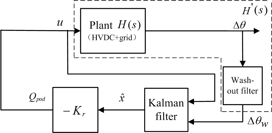
Fig. 2 shows the proposed LQG POD. The classic POD wash-out filter is added in LQG POD controller to avoid steady-state error. Q I, R 10−4; W I, V 10−2 in this case. The transfer matrix of regulator is:
$$Q_{pod} – K_r x – K_r sI – ALC^{-1} \begin{bmatrix} B & L \end{bmatrix} \begin{bmatrix} u \\ \Delta \theta_w \end{bmatrix}\tag{7}$$
1.1. Mixed sensitivity H∞ based on LMI
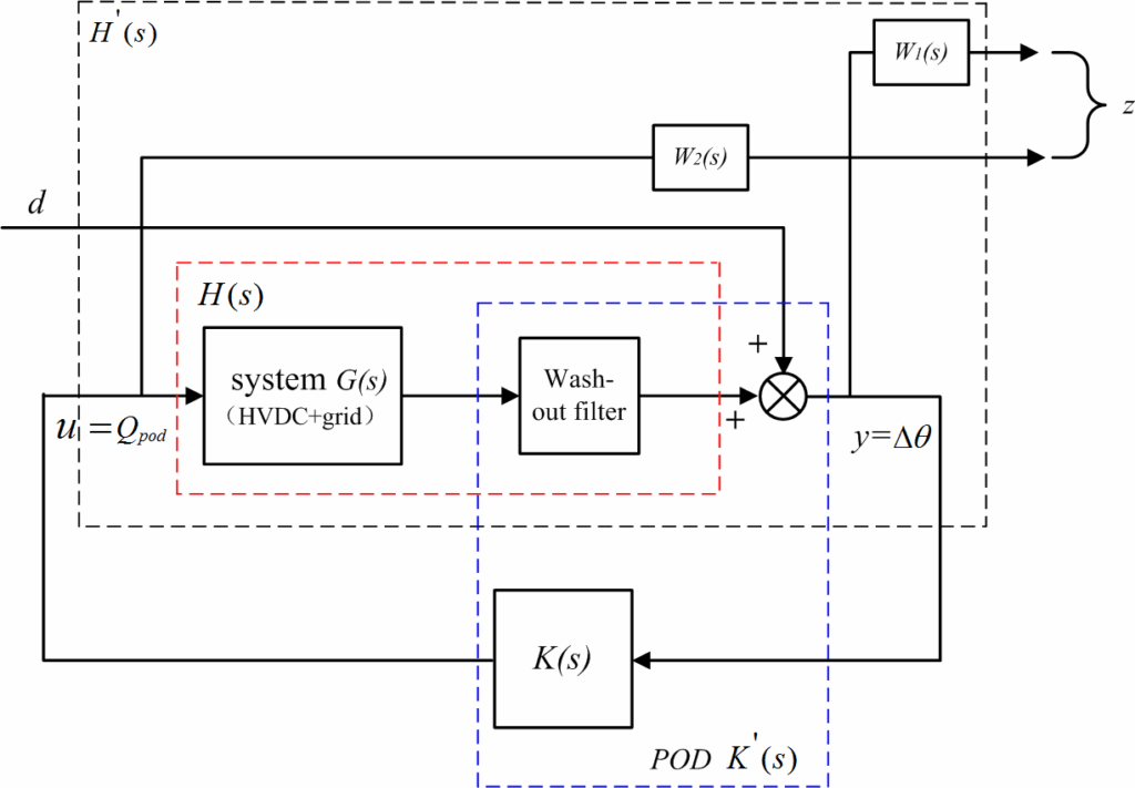
The interest of this approach lies in the clarity of its formal- ism and the physical interpretation of the synthesis criterion since it is defined by a transfer function or even a block diagram showing weights placed on the physical inputs and output signals of the system and this independently of the norm that one wishes to minimize (H2 or H∞ ). This formulation is conducive to the introduction of frequency weights on some signals (e.g., the control) to satisfy frequency specifications (e.g., the roll-off at high frequencies) for which the optimal LQG-type approach is poor (note however that the frequency LQG approach proposed a solution since the beginning of the 70’s to take into account frequency specifications. Particular standard forms (notably the mixed sensitivity presented in Fig. 3) have been studied and are directly adapted to the formulation of frequency robustness specifications on sensitivity functions. We show here how to formalize the mixed ”S KS ” synthesis problem for our application. For that we use frequency weights: W1 for S and W2 for KS . The H∞ problem consists of minimizing:
$$\left\|\begin{bmatrix} W_1 s S_s \\ W_2 s K S_s \end{bmatrix}\right\|_{\infty} < \gamma,\tag{8}$$
where γ denotes a positive real number. We consider the disturbance d as the only disturbance in the system (Fig. 3). W1 s and W2 s are the stability and performance specifications respectively and take the following forms [27]:
$$W_1 s = \frac{s\sqrt[k]{M_s} \, \omega_{b_k}}{s \, \omega_b \, \sqrt[k]{\varepsilon}}, \quad W_2 s = \frac{s \, \omega_{bc} \, \sqrt[k]{M_{nk}}}{\sqrt[k]{\varepsilon_1} s \, \omega_{bc}}\tag{9}$$
where the bandwidth are ωb 0.628 rad/sec, ωbc 12.56 rad/sec. Ms, Mn are defined for the peak sensitivity and ε 0.1, ε1 0.1 for the steady state error. k is the order of the weighting function. The target damping is set to ξdesired 10% for all the modes, as was the case for the design of classic POD. Thus, β 168◦ (β is the angle of conics in left complex plane directly correlated with damping ratio \(\xi \cos\left(\frac{\beta}{2}\right)\)
The different matrices are combined into a single system, called the augmented system. It is defined by the following state equations:
$$\left\{ \begin{array}{l} x_p = A_p x_p + B_{p1}d + B_{p2}u \\ z = C_1 x_p + D_{p11} d \\ y = C_2 x_p + D_{p21} d \end{array} \right.\tag{10}$$
be a stable representation of the augmented plant H′s of Fig. 3.
The state space parameters of controller Ks are Ak, Bk, Ck and Dk which can be found via solving LMIs (11), (12), (13).
$$\left[\begin{array}{cc} Q & I \\ I & S \end{array}\right] < 0
\tag{11}$$
$$\left[\begin{array}{cc} \Pi_{11} & \Pi_{21}^{T} \\ \Pi_{21} & \Pi_{22} \end{array}\right] < 0\tag{12}$$
$$\eta \otimes \Psi \, \eta^T \otimes \Psi^T < 0 \tag{13}$$
Where
$$\eta \begin{bmatrix} \sin \frac{\beta}{2} & \cos \frac{\beta}{2} \\ -\cos \frac{\beta}{2} & \sin \frac{\beta}{2} \end{bmatrix}, \tag{14}$$
⊗ is the Kronecker product, Q and S are obtained by solving the following Π11, Π21, Π22 and Ψ.
$$\Pi_{11} = \left[ \begin{array}{ccc} A_p Q & Q A_p^T & B_{p2} C \\ C^T & B_{p2}^T B_{p2} & B_{p1} \\ B_{p1} & B_{p2} D D_{p21} & -\gamma I \end{array} \right]\tag{15}$$
$$\Pi_{21} = \left[ \begin{array}{ccc} A & A_p & B_{p2} D C_{p2}^T \\ C_{p1} Q & D_{p12} C & S B_{p1} \\ D_{p11} & D_{p12} D D_{p21} & B D_{p21} \end{array} \right]
\tag{16}$$
$$\Pi_{22} = \left[ \begin{array}{ccc} A_p^T S & S A_p & B C_{p2} \\ C_{p1} & D_{p12} D C_{p2} & C_{p1} D_{p12} D C_{p2}^T \\ & & -\gamma I \end{array} \right]\tag{17}$$
$$\Psi = \left[ \begin{array}{ccc} A_p Q & B_{p2} C & A_p \\ B_{p2} D C_{p2} & S A_p & B C_{p2} \\ A & & \end{array} \right]\tag{18}$$
A state-space representation of the controller Ks is
$$D_k = D;\tag{19}$$
$$C_k = C – D_k C_2 Q M^T{}^{-1};\tag{20}$$
$$B_k = N^{-1} B – S B_{p2} D_k;\tag{21}$$
$$A_k = N^{-1} A – S A B_{p2} D_k C_{p2} Q M^T{}^{-1} – B_k C_{p2} Q M^T{}^{-1} – N^{-1} S B_{p2} C_k.\tag{22}$$
by solving LMIs (19) to (22), Q, S and A, B, C, D are calcu- lated, and M and N are given by
$$MN^{T}I – RS.\tag{23}$$
4. Proposed H∞ RSOFC based on model-matching
4.1. Selection of reference model
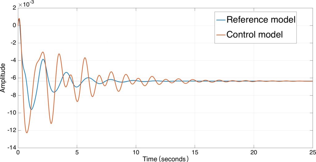
The nominal (or reference) model is a realization in the state space and selected in order to give desired damping (over 10%) (cf. Fig. 4) and stable zeros (see details in [21]). It is possible to write the state model in the following form.

$$\begin{cases} x_r = A_r x_r + B_r u_r \\ y_r = C_r x_r \end{cases}\tag{24}$$
The reference model and open-loop comparison validation is shown in Fig. 5. The proposed H∞ RSOFC based on model-matching is given in Fig. 6.
Based on (1) and (24), the augmented system is defined by the following state equations (cf. Fig. 6).
$$\begin{cases} X = AX + B_uc + B_r u_r \\ e = C_e X \end{cases}\tag{25}$$
where the controlled output is given by e y _ yr and X [ x xr e ]T .
$$A \begin{bmatrix} A & 0 & 0 \\ 0 & A_r & 0 \\ CA & -C_r A_r & 0 \end{bmatrix}, \quad B \begin{bmatrix} B \\ 0 \\ CB \end{bmatrix}, \quad B_r \begin{bmatrix} B \\ B_r \\ CB – C_r B_r \end{bmatrix}, \quad C_e \begin{bmatrix} 0 & 0 & I \end{bmatrix}\tag{26}$$
In this paper, the proposed H∞ RSOFC is defined by
$$u_c = Ke,\tag{27}$$
where K are the controller gains.
From (25), (26) and (27), the closed-loop system is given by ,
$$\begin{cases}
X = AX + B_r u_r \\
e = C_e X
\end{cases}\tag{28}$$
4.2. Proposed H∞ RSOFC stability and robustness analysis
The conditions of global asymptotic stability to determine the controller gains so that the system (28) is robust is studied in this subsection. This leads to the conditions expressed in Theorem 1.
Theorem 1: The robust control system in the form (28) under the control law (27) is asymptotically stable if and only if X XT > 0 and Y and below LMIs are verified
$$\min \gamma \tag{29}$$
subject to
$$\left[\begin{array}{ccc|c|c}
AX & XA^{T} & BY & Y^{T}B^{T} & B_r & C_e * X^{T} \\
B_r^{T} & -\gamma I & 0 \\
C_e * X & 0 & -\gamma I
\end{array}\right] < 0, \quad X > 0 \tag{30}$$
Then, based on (30), the controller gains (27) are ob- tained.
$$K = XY^{-1} \tag{31}$$
Proof. The proof of Theorem 1 is established by using the disturbance ur to the output e Transfer Function (TF).
$$T_{u_r e}s\, C_e sI – ABK^{-1}B_r \tag{32}$$
By minimizing the H∞ norm of (32) (||Ture||∞ ≤ γ), the rejection of external disturbances is obtained. Based on bounded real lemma ([17, 28]), the robust control system in the form of a (28) is stable, if and only if the matrix P PT > 0 is symmetric positive definite and the following LMIs are verified
$$\left[\begin{array}{ccc}
A^{T}PA & PB_r & C_e^{T} \\
B_r^{T}P & -\gamma I & 0 \\
C_e & 0 & -\gamma I
\end{array}\right] < 0 \tag{33}$$
$$\left[\begin{array}{ccc}
\phi & PB_r & C_e^{T} \\
B_r^{T}P & -\gamma I & 0 \\
C_e & 0 & -\gamma I
\end{array}\right] < 0, \tag{34}$$
where ϕ A B[0 0 k]T P PA B[0 0 k]. Define.
$$T \left[\begin{array}{ccc}
P^{-1} & 0 & 0 \\
0 & I & 0 \\
0 & 0 & I
\end{array}\right] \tag{35}$$
where I is the identity matrix. Multiplying left and right sides of the (34) by T and TT , respectively, with X KY , X P−1, the stability conditions (29) and (30) in Theorem 1 are obtained.
5. Proposed H∞ DDOFC based on model-matching
To avoid to run the reference model in real-time in order to produce the e signal in the controller, a an output-feedback is proposed. The structure of the resulting model-matching robust H∞ DDOFC is given in Fig. 7.
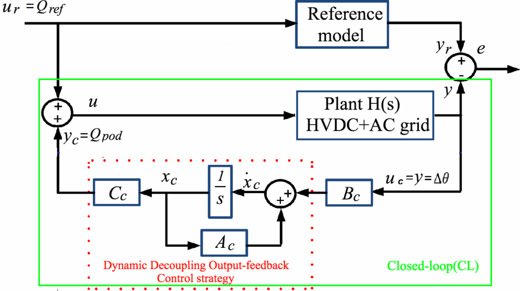
The proposed H∞ DDOFC dynamic equations are given by the following form
$$\begin{bmatrix} x_c & A_cx_c & B_cu_c \\ y_c & C_cx_c \end{bmatrix}\tag{36}$$
From Fig. 7, it follows,
$$\begin{bmatrix} u & u_r – u_c & u_r – y_c & u_r – C_cx_c \\ u_c & y & Cx \end{bmatrix}\tag{37}$$
From (1), (24) and (36), the virtual system state-space equation is
$$\begin{bmatrix} X & AX & B_ru_r \\ Y & CX & \end{bmatrix},\tag{38}$$
where \(Xt = \begin{bmatrix} x \\ x_r \\ x_c \end{bmatrix}^{T}\) and \(A = \begin{bmatrix} A & 0 & -BC_c \\ 0 & A_r & 0 \\ B_cC & 0 & A_c \end{bmatrix}, \quad B = \begin{bmatrix} B \\ B_r \\ 0 \end{bmatrix}, \quad C = \begin{bmatrix} -C & C_r & 0 \end{bmatrix}^{T}.\)
5.1. Proposed H∞ DDOFC stability and robustness analysis
Theorem 2: The virtual system (VS ) in the form (38) subject to the proposed H∞ DDOFC dynamic law (36) is asymptotically stable if and only if the matrcies Q, Z ∈ ℜnnr ×nnr are symmetric positive definite , Aˆ, ˆB, Cˆ ∈ ℜnnr ×nnr , are non singular and scalar γ, and below LMIs are verified,
$$\min \gamma \tag{39}$$
$$\left[\begin{array}{cccc} \phi_1 & \phi_1^T & \hat{A}^T\begin{bmatrix} A & 0 \\ 0 & A_r \end{bmatrix} & Q\begin{bmatrix} -C^T \\ C_r^T \end{bmatrix} \\ * & \phi_2 & \phi_2^T & Z\hat{B}\begin{bmatrix} B \\ B_r \end{bmatrix} \\ * & * & -\gamma I & 0 \\ * & * & 0 & -\gamma I \end{array}\right] \leq 0\tag{40}$$
$$\left[ \begin{array}{cc} Q & I \\ I & Z \end{array} \right] \geq 0\tag{41}$$
where
$$\phi_1 \begin{bmatrix} A & 0 \\ 0 & A_r \end{bmatrix} Q \begin{bmatrix} -B\hat{C} \\ 0 \end{bmatrix}, \quad \phi_2 Z \begin{bmatrix} A & 0 \\ 0 & A_r \end{bmatrix} \begin{bmatrix} B\hat{B}\hat{C} \\ 0 \end{bmatrix}^T,$$
Therefore, by solving LMIs (40)-(41), the H ∞DDOFC parameters can be written as follows:
$$A_c = N^{-1} A M^{-T}, \quad B_c = N^{-1} \hat{B}, \quad C_c = \hat{C} M^{-T},\tag{42}$$
where
$$A\widehat{A} – Z\begin{bmatrix} A & 0 \\ 0 & A_r \end{bmatrix}Q – N\begin{bmatrix} B_c C \\ 0 \end{bmatrix}^T Q – Z\begin{bmatrix} BC_c \\ 0 \end{bmatrix}M^T\tag{43}$$
and
$$NM = I – ZQ.\tag{44}$$
Proof. By minimizing the H norm of (32) (||Ture||∞ ≤ γ), the rejection of external disturbances is obtained. Based on bounded real lemma ([17], [28]), the robust control system in the form of a (36) is stable, if and only if the matrix W ∈ ℜ2nnr ×2nnr is symmetric positive definite and LMIs are satisfied,
$$\begin{bmatrix} A^T W + WA & WB & C^T \\ B^T W & -\gamma I & 0 \\ C & 0 & -\gamma I \end{bmatrix} \leq 0
\tag{45}$$
$$W \geq 0.\tag{46}$$
Based on Schur complement method [29]- [32] using W and W−1 , we have;
$$W \begin{bmatrix} Z & N \\ N^T & \star \end{bmatrix}, \quad W^{-1} \begin{bmatrix} Q & M \\ M^T & \star \end{bmatrix}\tag{47}$$
where ⋆ is unknown matrix. Let
$$1\begin{bmatrix} Q & I \\ M^T & 0 \end{bmatrix}, 2\begin{bmatrix} I & Z \\ 0 & N^T \end{bmatrix}
\tag{48}$$
From WW−1 I , it can be inferred
$$2W_1\tag{49}$$
In this case,
$${}^T_2 WA {}^T_2 A_1\tag{50}$$
So that,
$${}^T_2 A_1 \begin{bmatrix} I & 0 \\ Z & N \end{bmatrix} \begin{bmatrix} A & 0 & -BC_c \\ C & A_r & 0 \\ B_c C & 0 & A_c \end{bmatrix} \begin{bmatrix} Q & I \\ M^T & 0 \end{bmatrix} \left[ \begin{bmatrix} A & 0 \\ 0 & A_r \end{bmatrix} Q \begin{bmatrix} -BB_c \\ 0 \end{bmatrix} M^T \right] \begin{bmatrix} A & 0 \\ 0 & A_r \end{bmatrix} Q_1 Q_2\tag{51}$$
and,
$${}^T_1 WB \, {}^T_2 B_1 \begin{bmatrix} I & 0 \\ Z & N \end{bmatrix} \begin{bmatrix} B \\ B_r \\ 0 \end{bmatrix} \begin{bmatrix} B \\ B_r \end{bmatrix} Z \begin{bmatrix} B \\ B_r \end{bmatrix}\tag{52}$$
Then,
$${}^T_1 C \left[ \left[ -C \quad C_r \right] C \right] \begin{bmatrix} Q \\ M^T \end{bmatrix} \begin{bmatrix} I \\ 0 \end{bmatrix}^T \begin{bmatrix} Q \begin{bmatrix} -C^T \\ C_r^T \end{bmatrix} \\ -C^T_r \\ C_r^T \end{bmatrix}
\tag{53}$$
where,
$$Q_1 Z \begin{bmatrix} A & 0 \\ 0 & A_r \end{bmatrix} Q N \begin{bmatrix} B_c & C & 0 \end{bmatrix} Q Z \begin{bmatrix} -BC_c \\ 0 \end{bmatrix} M^T, \quad N A_c M^T, \quad Q_2 Z \begin{bmatrix} A & 0 \\ 0 & A_r \end{bmatrix} N \begin{bmatrix} B_c & C & 0 \end{bmatrix}\tag{54}$$
Thus,
$$A Z \begin{bmatrix} A & 0 \\ 0 & A_r \end{bmatrix} Q N \begin{bmatrix} B_c & C & 0 \end{bmatrix} Q Z \begin{bmatrix} -BC_c \\ 0 \end{bmatrix} M^T, \quad N A_c M^T, \quad B N B_c, \quad C C_c M^T\tag{55}$$
Therefore, (45) and (46) are equivalent to (40) and (41).
6. Validation Tests
In this section, RSOFC and DDOFC controllers depicted in Sections 4 and 5 are validated in linearized full model and nonlinear model and compared with the other controllers presented in Sections 2 and 3.
6.1. Linearized model validation
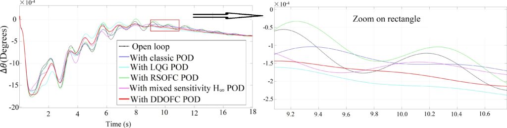
The model tested in this section is the linearized model from EUROSTAG and tested in Matlab with a step disturbance on angle difference ∆θ. They are shown in Fig. 8. The modes can be identified by measuring their frequency from two peaks. The description of these results are shown below:
- at t 8s, mode 2: compared to the classic POD and RSOFC, DDOFC POD and LQG POD give better damping
- from t 2s to 4s, mode 5: The performance of DDOFC POD, LQG POD, and mixed sensitivity H∞POD give less undershoot and sufficient damping.
- from t 1s to 3s, mode 1 (in zoomed figure of open-loop curve): Only observed in the curve with LQG.
Based on Table 2 analysis, it can be observed that, the proposed DDOFC POD gives the desired target damping of modes 1 and 2 without disturbing the others and a better damping in a wide range frequency band. The damping for each mode is over 10% for DDOFC POD, LQG POD, and H∞POD while the classic POD enhance the damping of mode 2, but encumber mode 4. Mode 3 damping is reached highest value for LQG POD but it’s acceptable for mixed sensitivity POD during mode 4 and 5. On the other hand, damping for each mode is decreased excepting for mode 5 when RSOFC is used.
6.2. Nonlinear system validation
The study and robustness analysis is more difficult due to the system nonlinearities. In addition, each response curve is the result of several modes mixed with a nonlinear dynamic. It is therefore difficult to highlight each mode individually. Disturbance scenarios must be well chosen. Moreover, the observability of the modes depends on the selected output signal. To validate the performance and robustness of the proposed controllers, two situations are considered: for the first one, called nominal operation case, the simulations are carried with the same grid situation considered for the synthesis of the controllers. For the second one, called robust operation case, the grid is disturbed (with load variations, line/generators tripping) for simulation without recomputing the controllers.
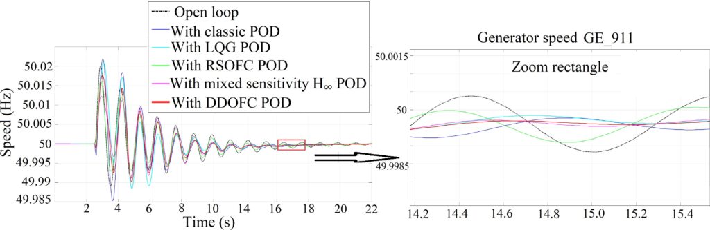
The performances and robustness of proposed strategies are validated on nonlinear model with Eurostag software. A short-circuit is performed at generator GE_918 terminal bus. Due to the fact that generator GE_918 is closed to GE_911, which is the most participating machine in mode 2 (ff.Table 1), this disturbance excites the modes of interest.
6.2.1. Nominal operation case
Fig. 9 shows the response of the proposed strategies in the nominal operation case.
According to the zoom of Fig. 9, one can see that for mode 2 (we recognize it by measuring the frequency be- tween the peaks of the curves from the oscillation 8th), the DDOFC, the mixed sensitivity H∞POD and LQG POD give more damping compared to RSOFC and classic POD. In addition, at t 3s, the contributions of several mixed modes with nonlinear dynamics are observable. Moreover, be- tween the 4th and 8th oscillations (the period during which mode 1 can be observed), (cf. table 2).
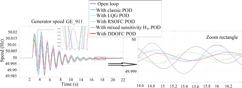
6.2.2. Robust operation cases
Different disturbed grid situations are considered to validate the proposed strategies in uncertainties case. These cases correspond to the robustness issue: variation of some of its parameters – called parametric robustness (see details in [22]). Responses obtained with the same controllers considered above are now shown in Fig. 10, 11, 12, 13.
- Reverse power flow case (in Fig. 10)
- at t 12s (mode 2): RSOFC POD and mixed sensitivity H∞ POD give more damping.
- From oscillation 3rd (mode 4): Although the RSOFC POD give more damping compared to the other controllers, but it gives insufficient damping nominal operation case.
- from t 3s to t 5s: With the mixed sensitivity H∞ the POD gives small oscillation at t 3.5s (cf. 10).
- Increased load case (in Fig. 11)
Table 2: Comparison of damping
No. | damping (ξ) without POD (%) | damping (ξ) with classic POD (%) | damping (ξ) with LQG POD (%) | damping (ξ) with Mixed sensitivity H∞ POD(%) | damping (ξ) with RSOFC POD (%) | damping (ξ) with DDOFC POD(%) |
1 | 19.5 | 30.5 | 21.7 | 20.29 | 18.6 | 23.3 |
2 | 4.5 | 6.1 | 10.9 | 11.67 | 4.2 | 12.6 |
3 | 10.1 | 12.0 | 14.9 | 12.33 | 9.6 | 10.8 |
4 | 8.3 | 8.1 | 11.4 | 12.41 | 7.9 | 10.6 |
5 | 10.1 | 12.4 | 13.6 | 14.97 | 14.2 | 14.1 |
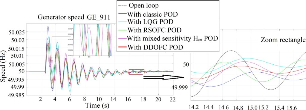
- at t 12s (mode 2): H∞, LQG and DDOFC POD give the same acceptable damping.
- From the oscillation 3rd to 5th: the damping provided by the H∞POD is not sufficient for mode 4. In addition, the overshoot with LQG POD in the first oscillation is undesirable.
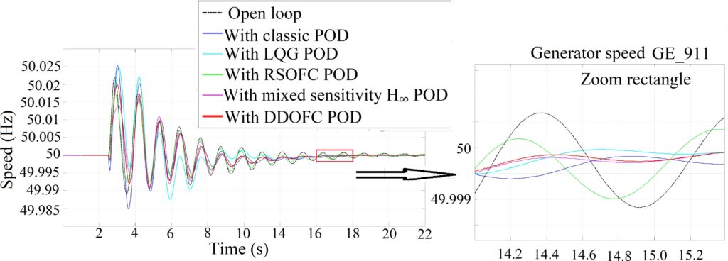
- Tripping generator case (in Fig. 12)
- During the first two oscillations: the POD LQG as well as the classic POD even increase the oscillations during the first two swings.
- From t 12s (mode 2): The DDOFC, the mixed sensitivity H∞ and the LQG POD, have more damping compared to the other controllers.
- DDOFC POD gives more damping than the other controllers during the 3th to the 6th swing (mode 1).
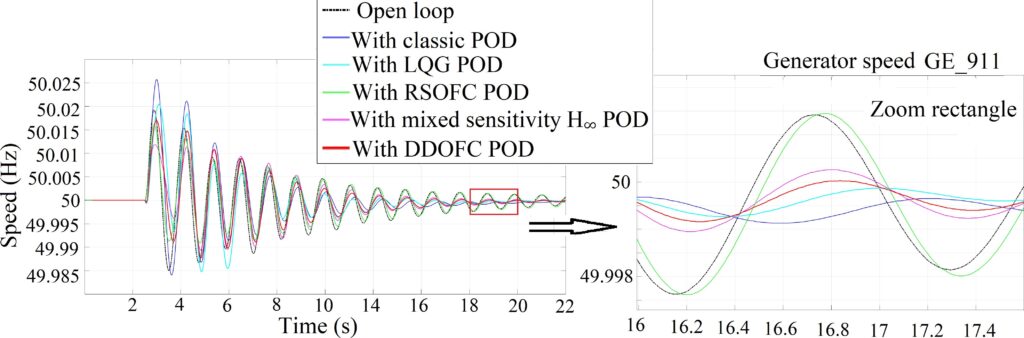
• Tripping lines case ( In Fig. 13)
- 4th to 8th oscillation (mode 1): Classic, LQG, and DDOFC POD give more damping during the 4th to the 8th swing (mode 1).
- In the zoomed figure (mode 2), the damping is greater with the DDOFC than with the mixed sensitivity H∞ and the RSOFC POD.
- The overshooths is greater with LQG POD than with open-loop during the first two swings.
In summary, the proposed DDOFC POD is more robust- ness and better damping for all the cases.
7. Conclusion
In this paper two robust model-matching based POD are studied. Sufficient conditions are derived for robust stabilization, in the sense of Lyapunov method and based on a reference model and have been formulated using an LMI format to obtain the controllers’ gains. The robustness of the proposed controller is finally tested and compared to LQG, mixed sensitivity H∞ and standard (IEEE) POD controllers on a realistic benchmark of 19 generators connected by a meshed AC grid.
Paper contributions are: (i) improves damping and robustness subject to the unstable zeros compared with standard controller structures (LQG, mixed sensitivity H∞ and standard POD controllers); (ii) the proposed controller is validated using Eurostag, which is an industrial software for grid dynamics ; (iii) it can be easily implemented in real case and it consists in a simple output-feedback.
The control methodology is applied here for Q modulation but can be extended to coordinate P and Q modulation of the HVDC link.
It is planned in the near future to implement the overall proposed control strategy on the France-Spain and France- Italy HVDC interconnection in real grid situations.
8. Appendix
8.1. LQG controller:
Based on LQG 3.1, the gains are given by:
L=[-164.18 47.48 80.33 57.635 96.34 -19.51 2.81 48.01
35.078 8.58 -7.82 -0.33 -9.20T ;
Kr= [ 13.7682 -3.3704 -4.0354 6.5771 7.0691 4.3546 2.4524
-1.5362 1.1628 0.7133 -0.4256 -0.6244 -0.5161].
u to Qpod Transfer Function(TF) is H1, and TF fomr ∆θ to u is
H2:
$$H_1^{\substack{n-1 \\ n}}{\substack{i0 \\ j0}} \frac{N1{is}}{D1_{js}} = \frac{N1_{n-1\,s_n} \cdots N1_{1s} \, N1_0}{D1_{n\,s_n} \cdots D1_{1s} \, D1_0}\tag{56}$$
$$H_2 = \frac{N2_{n-1}s^{n-1} \ \ldots\ N2_1s\ N2_0}{D2_n s^n \ \ldots\ D2_1s\ D2_0}\tag{57}$$
n 13 (including the wash-out filter (dimension 1))(cf. Table 3).
Table 3: TF of LQG POD paramaters
i,j= | N1 | D1 | N2 | D2 |
13 | / | 1 | / | 1 |
12 | -3.681 | 43.19 | 1781 | 43.19 |
11 | -189.3 | 785.2 | 1.814e04 | 785.2 |
10 | -3051 | 1.092e04 | 3.614e05 | 1.092e04 |
9 | -3.894e04 | 1.087e05 | 2.343e06 | 1.087e05 |
8 | -3.575e05 | 8.942e05 | 2.358e07 | 8.942e05 |
7 | -2.571e06 | 5.837e06 | 9.686e07 | 5.837e06 |
6 | -1.513e07 | 3.203e07 | 6.336e08 | 3.203e07 |
5 | -7.04e07 | 1.431e08 | 1.381e09 | 1.431e08 |
4 | -2.672e08 | 5.266e08 | 6.488e09 | 5.266e08 |
3 | -8.032e08 | 1.557e09 | -3.658e08 | 1.557e09 |
2 | -1.735e09 | 3.469e09 | 5.733e09 | 3.469e09 |
1 | -2.923e09 | 5.716e09 | -9.87e10 | 5.716e09 |
0 | -1.42e09 | 4.454e09 | -1.387e11 | 4.454e09 |
8.2. Mixed sensitivity H∞ controller:
The H∞ controller TF in 3.2 is:
$$Ks = \frac{N_{n-1}s^{n-1} \ \ldots\ N_1s\ N_0}{D_n s^n \ \ldots\ D_1s\ D_0}\tag{58}$$
In (58), n 15 (including the wash-out filter (dimension 1) and frequency weights (dimension 2)). H∞ controller parameters are given in Table 4
Table 4: TF of H∞ POD paramaters
i= | N | D |
15 | / | 1 |
14 | 9.4e05 | 4.6e05 |
13 | 9.4e7 | 7.8e06 |
12 | 1.1e9 | 1.5e08 |
11 | 1.9e10 | 1.5e09 |
10 | 1.38e11 | 1.5e10 |
9 | 1.3e12 | 9.8e10 |
8 | 5.95e12 | 6.3e11 |
7 | 3.51e13 | 2.91e12 |
6 | 1.1e14 | 1.3e13 |
5 | 4.3e14 | 3.9e13 |
4 | 7.4e14 | 1.17e14 |
3 | 1.8e15 | 2.15e14 |
2 | 1.1e15 | 3.9e14 |
1 | -3.3e13 | 2.6e14 |
0 | 3.3e14 | 1.1e13 |
8.3. Reference model:
The reference model TF used in proposed two controller:
$$f_r s \frac{N r_{n-1} s^{n-1} \dots N r_1 s \; N r_0}{D r_n s^n \dots D r_1 s \; D r_0}\tag{59}$$
n 12 (cf. Table 5).
Table 5: Reference model TF
i= | Nr | Dr |
12 | / | 1 |
11 | 0.02143 | 19.54 |
10 | 0.1264 | 355.5 |
9 | 0.9629 | 3773 |
8 | – 1.255 | 3.6e4 |
7 | – 126.5 | 2.5e5 |
6 | – 1088 | 1.6e6 |
5 | – 9771 | 7.2e6 |
4 | – 5.1e4 | 3.1e7 |
3 | – 2.3e5 | 9.2e7 |
2 | – 8.7e5 | 2.7e8 |
1 | – 1.8e6 | 4.1e8 |
0 | – 4.7e6 | 7.3e8 |
8.4. ROSCF controller:
The gains calculated in (31): Y=1.150696148547366e-12; X=2.009746646814367e-13.
Then, the gain of the controller is: K 5.725578148724988. Notice that the dimension of the ROSCF controller is 13 (equal to the dimension of the reference model (12) + the one of the wash-out filter (1)).
8.5. DDOFC controller:
The transfer function of controller DDOFC Ks:
$$K s \frac{N d_{n-1} s^{n-1} \dots N d_1 s \; N d_0}{D d_n s^n \dots D d_1 s \; D d_0}\tag{60}$$
Since the order of the controller depends on the control model plus reference model, n 26 (dimension of the plant (12) + dimension of the reference model (12) + wash-out filters for the plant and reference model (2)). Parameters are shown in Table 6.
Table 6: Transfer function of DDOFC POD paramaters
i= | Nd | Dd |
26 | / | 1 |
25 | 5.267e05 | 4.057e04 |
24 | 1.713e07 | 1.465e06 |
23 | 4.532e08 | 4.032e07 |
22 | 8.033e09 | 7.692e08 |
21 | 1.225e11 | 1.234e10 |
20 | 1.496e12 | 1.621e11 |
19 | 1.616e13 | 1.865e12 |
18 | 1.481e14 | 1.856e13 |
17 | 1.217e15 | 1.65e14 |
16 | 8.672e15 | 1.3e15 |
15 | 5.573e16 | 9.242e15 |
14 | 3.119e17 | 5.888e16 |
13 | 1.568e18 | 3.402e17 |
12 | 6.764e18 | 1.768e18 |
11 | 2.567e19 | 8.326e18 |
10 | 7.833e19 | 3.519e19 |
9 | 1.879e20 | 1.341e20 |
8 | 1.951e20 | 4.546e20 |
7 | – 7.141e20 | 1.372e21 |
6 | – 6.079e21 | 3.617e21 |
5 | – 2.359e22 | 8.277e21 |
4 | – 6.919e22 | 1.593e22 |
3 | -1.507e23 | 2.516e22 |
2 | – 2.483e23 | 3.057e22 |
1 | – 2.907e23 | 2.551e22 |
0 | – 1.568e23 | 1.08e22 |
- EWEA, Pure power – wind energy targets for 2020 and 2030,” tech. rep,
EWEA, 2009. - EWEA, Oceans of opportunity – harnessing Europe’s largest domestic energy resource offshore,” tech. rep., EWEA, September 2009.
- C. Du, The control of VSC-HVDC and its use for large industrial power systems. PhD thesis, Departament of Electric Power Engineering, Chalmers University of Technology, Goteborg, Sweden, 2003.
- M. P. Bahrman, Hvdc transmission overview,” IEEE, pp. 1-7, 2008
- L. Arioua, B. Marinescu, Robust grid oriented control of high voltage DC links embedded in an AC transmission system[J]. International Journal of Robust and Nonlinear Control, 2016, 26(9): 1944-1961.
- L. Arioua, B. Marinescu, Multivariable control with grid objectives of an HVDC link embedded in a large-scale AC grid[J]. International Journal of Electrical Power and Energy Systems, 2015, 72: 99-108.
- D. Lee, IEEE recommended practice for excitation system models for power system stability studies (ieee std 421.5-1992)[J]. Energy Development and Power Generating Committee of the Power Engineering Society, 1992, 95(96).
- S. Skogestad, I. Postlethwaite, Multivariable feedback control: analysis and design[M]. New York: Wiley, 2007.
- D. Mondal, A. Chakrabarti, and A. Sengupta. ”LMI based wide area TCSC controller in mitigating small signal oscillations.” Int. J. of Soft Computing and Engineering, IJSCE 6.1 (2012): 139-144.
- B. Marinescu, D. Petesch, (2014). Three-level coordination in power system stabilization. Electric Power Systems Research, 111, 40-51.
- J. Li, J. Lu, W. Su, Optimal output feedback control of a class of linear systems with quasi-colored control-dependent multiplicative noise, Preprint https://arxiv.org/abs/2109.01358, 2021.
- S. I. Eom, E. J. Kim, T. Y. Shin, M. H. Lee and F. Harashima, The ro- bust controller design for lateral control of vehicles. In Proceedings 2003 IEEE/ASME International Conference on Advanced Intelligent Mechatron- ics (AIM 2003), volume 1, pp. 570–573, 2003.
- M. Shimakage, S. Satoh, K. Uenuma and H. Mouri, Design of lane keeping control with steering torque input. JSAE review, vol. 23, no. 3, pp. 317–323, 2002.
- P. Apkarian, D. Noll, and A. Rondepierre, (2008). Mixed H2/Hin f ty control via nonsmooth optimization. SIAM Journal on Control and Optimization, vol. 47, no. 3, pp.1516-1546, 2008.
- S. Kanev, C. Scherer, M. Verhaegen, B. De Schutter, (2004). Robust output- feedback controller design via local BMI optimization. Automatica, 40(7), 1115-1127.
- D. Wang and C. Mu, Adaptive Robust H Infinity Control For Nonlinear Systems, Springer, 2022.
- F. Ferrante, C. Ravazzi and F. Dabbene, An LMI Approach for Structured H-infinity State Feedback Control, IFAC PapersOnLine 53-2, pp. 4058-4063, 2020.
- E. Kamal, A. Aitouche, R. Ghorbani and M. Bayart, Robust fuzzy logic con- trol of wind energy conversion systems with unknown inputs, International Journal of Power and Energy Systems, Control and Intelligent Systems, vol. 32, no.2, pp.71, 2012.
- E. Kamal, A. Aitouche, R. Ghorbani and M. Bayart, Intelligent control of WECS subject to parameter uncertainties, Actuator and Sensor Faults, Control and Intelligent Systems, vol. 40, no.3, pp.160, 2012.
- E. Kamal and A. Aitouche, Design of maximum power fuzzy controller for PV systems based on the LMI-based stability, Intelligent Systems in Technical and Medical Diagnostics. Advances in Intelligent Systems and Computing, vol. 230. Springer 2013, pp.77-88.
- Y. Xing, B. Marinescu and F. Xavier, Robust Research of Power Oscillations Damping Controller for HVDC Inserted in Meshed AC Grids, 2019 IEEE Milan PowerTech,pp. 1-6, 2019.
- Y. Xing, E. Kamal, B. Marinescu and F. Xavier. Advanced control to damp power oscillations with VSC-HVDC links inserted in meshed AC grids. International Transactions on Electrical Energy Systems, vol. 31, no. 12, pp.1-22., 2021.
- M. Belhocine, B. Marinescu, F. Xavier, Input signal and model structure analysis for the hvdc link pod control[C]//2017 IEEE Manchester PowerTech. IEEE, pp.1-6, 2017.
- Y. Xing, B. Marinescu, M. Belhocine, et al. Power oscillations damping con- troller for hvdc inserted in meshed ac grids[C]//2018 IEEE PES Innovative Smart Grid Technologies Conference Europe (ISGT-Europe), pp.1-6, 2018.
- D. T. Nguyen, D. Georges, et Q. T. Tran, An Energy Approach to Optimal Selection of Controllers and Sensors in Power System, International Journal of Emerging Electric Power Systems, Berkeley Electronic Press, Vol. 9, 2008, http://www.bepress.com/ijeeps/vol9/iss6/art2.
- Y. Xing, M. P. Aghababa, B. Marinescu and F. Xavier, F. [C]. Analysis and Control of Non-Minimum Phase Behavior in Nonlinear AC Grids Equipped with HVDC Links. In 2019 IEEE PES Innovative Smart Grid Technologies Europe (ISGT-Europe)(2019, September)
- K. Zhou, J C. Doyle, Essentials of robust control [M]. Upper Saddle River, NJ: Prentice hall, 1998.
- Duan, Guang-Ren, and H-H. Yu. [M]. LMIs in control systems: analysis, design and applications. CRC press, 2013.
- E Kamal, M Bayart and A Aitouche, Robust control of wind energy conver- sion systems, 2011 International Conference on Communications, Comput- ing and Control Applications (CCCA), pp.1-6, 2011
- N. Ouddah, L. Adouane, R. Abdrakhmanov and E. Kamal, Optimal Energy Management Strategy of Plug-in Hybrid Electric Bus in Urban Conditions, Proceedings of the 14th International Conference on Informatics in Control,(ICINCO 2017), vol1, pp. 304-311, 2017
- E. Kamal, A. El Hajjaji and A. M. Mabwe, State of charge estimation based on extened Kalman filter algorithm for Lithium-Ion battery, 2015 23rd Mediterranean Conference on Control and Automation (MED), June 16-19, Torremolinos, Spain, pp. 734-739, 2015.
- J. Cha, S. Kang and S. Ko, Infinite Horizon Optimal Output Feedback Con- trol for Linear Systems with State Equality Constraints. Int. J. Aeronaut.
Space Sci., vol. 20, pp. 483-492, 2019.
No related articles were found.