Machine-Learning based Decoding of Surface Code Syndromes in Quantum Error Correction
(This article belongs to the Special Issue on Special Issue on Multidisciplinary Sciences and Advanced Technology (SI-MSAT 2022) and the Section Applied Mathematics (APM))
Export Citations
Cite
Bhoumik, D. , Sen, P. , Majumdar, R. , Sur-Kolay, S. , KJ, L. K. and Iyengar, S. S. (2022). Machine-Learning based Decoding of Surface Code Syndromes in Quantum Error Correction. Journal of Engineering Research and Sciences, 1(6), 21–35. https://doi.org/10.55708/js0106004
Debasmita Bhoumik, Pinaki Sen, Ritajit Majumdar, Susmita Sur-Kolay, Latesh Kumar KJ and Sundaraja Sitharama Iyengar. "Machine-Learning based Decoding of Surface Code Syndromes in Quantum Error Correction." Journal of Engineering Research and Sciences 1, no. 6 (June 2022): 21–35. https://doi.org/10.55708/js0106004
D. Bhoumik, P. Sen, R. Majumdar, S. Sur-Kolay, L.K. KJ and S.S. Iyengar, "Machine-Learning based Decoding of Surface Code Syndromes in Quantum Error Correction," Journal of Engineering Research and Sciences, vol. 1, no. 6, pp. 21–35, Jun. 2022, doi: 10.55708/js0106004.
Errors in surface code have typically been decoded by Minimum Weight Perfect Matching (MWPM) bas -based Machine Learning (ML) techniques have been employed for this purpose, although how an ML decoder will behave in a more realistic asymmetric noise model has not been studied. In this article we (i) establish a methodology to formulate the surface code decoding problem as an ML classification problem, and (ii) propose a two-level (low and high) ML-based decoding scheme, where the first (low) level corrects errors on physical qubits and the second (high) level corrects any existing logical errors, for various noise models. Our results show that our proposed decoding method achieves ~10x and ~2x higher values of pseudo-threshold and threshold respectively, than for those with MWPM. We also empirically establish that usage of more sophisticated ML models with higher training/testing time, do not provide significant improvement in the decoder performance.
1. Introduction
Quantum computers are expected to provide faster and often more accurate solutions to some of the problems of interest such as factorization [1], database searching [2], Hamiltonian simulation [3], finding the lowest energy con- figuration of molecular systems [4]. Quantum computers make use of properties such as superposition, entangle- ment etc., which are not observed in macroscopic world, to achieve the speedup. A general quantum bit, or qubit, is mathematically represented as |ψ⟩=α |0⟩+β |1⟩, α, β ∈ C,
|α|2+|β|2=1 [5].
Quantum states are, however, very prone to errors. Being vectors in Hilbert space, even the slightest unwanted rotation occurring due to interaction with the environment introduces error in the quantum system. It was shown by [6], that any unitary quantum error can be expressed as a linear combination of the Pauli matrices (I, X, Y, Z) 1. Hence, if a quantum error correcting code (QECC) can correct the Pauli errors, then it can also correct any unitary error. The 9-qubit code [6], 7-qubit code [7] and 5-qubit code [8] are some early QECCs. The 5-qubit code is optimum in the number of qubits .
The circuit realization of the above-mentioned QECCs comprise multiple operations involving qubits which are not adjacent to each other. Operation on two non-adjacent qubits is both slow and error-prone, due to the multiple swap operations required. Surface code was introduced to overcome this drawback, known as the Nearest Neighbour (NN) problem, by placing the qubits in a 2D grid-like structure [9], and the operations for error correction are performed only between adjacent qubits. Protocols are formulated for error recovery, and the efficacy of these protocols were studied in [10] which is reviewed in a simplied manner by [11]. An improved decoding algorithm for the surface code is formulated in [12].
A QECC encodes n > 1 physical qubits into m < n logical qubits, where the latter are expected to be more secure under noise. A decoder (which is a classical process), on the other hand, detects the error present in the logical qubit. Decoding is followed by another step where the correction is applied physically and classically (or in some cases noted logically only [13]). A distance d QECC can correct \(\left\lfloor\frac{d}{2} \right\rfloor\)
errors on the physical qubits, keeping the logical qubit error free. However, the logical qubit can become erroneous as well if more errors occur. This is termed as logical error. The errors may occur due to interaction with the environment, or faulty decoding. While the first issue may be tackled with a QECC having a larger d, the latter can pose a serious threat towards building error corrected qubits. The performance of a decoder for a QECC is assessed by two parameters [14], namely: (i) pseudo-threshold, which is the probability of physical error below which error-correction leads to a lower logical error probability, and (ii) threshold, which is the probability of physical error beyond which increasing d leads to higher logical error probability.
Apart from the accuracy of decoding, the time required is also important. In a fault-tolerant quantum computer, the qubits are encoded only once at the beginning of the computation, whereas they are decoded several times during the computation. Therefore, decoding time is critical [5, 15]. The most popular decoding algorithm for surface codes is Blossom Decoder [16] based on O(N4) time Minimum Weight Perfect Matching (MWPM) algorithm, N being the number of qubits. Recently machine learning (ML) has been used for decoding in linear time [17]. A baseline decoding algorithms complemented by different kinds of deep neural decoders was introduced by [18] and applied to analyze the common fault-tolerant error correction protocols such as the surface code. The decoding problem is reduced to a classification problem that a feedforward neural network can solve, in [19], for small code distances. Reinforcement Learning based decoders for Fault-Tolerant Quantum Computation were proposed in [20]. It has been observed that the MWPM based decoder performs satisfactorily when the error probability of the system is low, as it always tries to find the minimum number of errors that can generate the observed syndrome (see Section II below). But occurrence of error(s) in the system during decoding is ignored, which the ML based approaches do consider. Therefore, ML based decoders are expected to perform at least as well as MWPM based method and in less time.
ML based decoders can tackle errors incorporated due to faulty decoding upto some extent. This is achieved by introducing two-level decoding, where the low level is a traditional decoder (need not be an ML decoder [19]), and the high level (necessarily ML decoder) predicts any logical errors that may have resulted during decoding. In [17] the authors have used ML for both low and high-level decoders. However, it is unclear whether their noise model considers errors in a single or multiple steps in the error correction cycle of surface code (see Fig: 2). Moreover, the performance of ML decoders for asymmetric noise (which is a more realistic noise model [21]), and whether the usage of more sophisticated ML models can significantly enhance the performance of the decoder, remains largely unanswered.
This article aims to address these unanswered problems by using machine learning based low and high level de- coders for both symmetric and asymmetric noise model. We want to emphasize here that the primary focus of this paper is the efficient mapping of the surface code decoding problem to ML classification, showing its decoding performance, and experimentally verifying whether the sophistication of the used ML model has any significant effect on the decoding performance. In this work we are applying machine learning for quantum error correction, hence the machine learning tasks are purely classical, not quantum. In other words, quantum machine learning is not involved in our approach. As a preliminary research, we have assumed that only the data qubits may be noisy, but both the measurement and the stabilizers are noise-free. In our follow-up work, we will consider noisy data, stabilizer, as well as non-ideal measurement.
The rest of the paper is organized as follows: we have summarized our contributions here in Section 2. In Section 3, we have outlined the stabilizer formulation of the surface code. In Section 4, we have established the formulation of the decoding problem of a surface code as an ML classification problem. In Section 5 we have presented our results with various error models and our concluding remarks appear in Section 6. In the Appendix we have provided the list of the acronyms used in this paper.
2. Summary of the contributions
The main contributions of our work are to:
- design a well-defined step-by-step methodology to formulate the decoding problem in surface code as an ML classification problem;
- study the performance of ML based low and high level decoders, for distance 3, 5 and 7 surface codes, where error can occur in one or more of the eight steps in the surface code QECC cycle with equal probability. We show that our ML based decoder achieves ∼ 10× higher pseudo-threshold and ∼ 2× higher threshold as compared with MWPM based decoder.
- establish that our ML-based decoder outperforms the one based on MWPM for varying degrees of asymmetry in the noise model as well;
- experimentally show that varying the level of sophistication (i.e., number of layers, nodes in each layer, etc.) for Feed Forward Neural Network (FFNN) and Convolutional Neural Network (CNN) does not pro- vide significant improvement in the performance of the syndrome decoder;
- show that when distance d is small, and hence the total number of distinct errors is also small, the ML based decoder can learn the most probable errors within a small subset of the training data, which is generated uniformly at random. Therefore, a small train-test ratio suffices to obtain a good decoding
- empirically determine the degree of asymmetry of the noise channel below which an ML decoder trained using symmetric noise model retains optimal pseudo threshold. This provides an estimate of re-usability of a pre-trained ML decoder on a variety of noise
3. Stabilizer Formulation of Surface Code
In [22], the author proposed the stabilizer formulation for error correction. A set of mutually commuting operators M1, . . . , Mr, where each Mi ∈ {I, X, Z, Y}⊗n, is said to stabilize an n-qubit quantum state |ψ⟩ if Mi |ψ⟩=|ψ⟩, ∀ i [22]. An error E is said to correctable by a QECC, if there exist stabilizers Me ⊆ {M1, . . . , Mr}, such that Me (E |ψ⟩) = −E |ψ⟩.
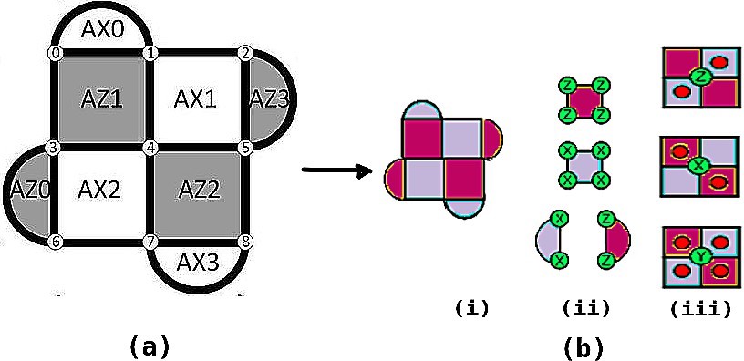
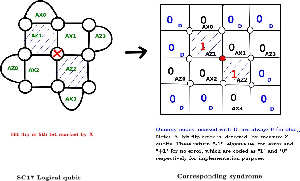
A QECC is called degenerate if there exist errors e1 ≠ e2 such that e1 |ψ⟩=e2 |ψ⟩ where |ψ⟩ is the codeword. It is not possible to distinguish between such errors in a degenerate code. Surface code is a degenerate stabilizer code. Surface code is implemented on a two-dimensional array of physical qubits. The data qubits (in which the quantum information is stored) are placed on the vertices, and the faces are the stabilizers (refer Fig. 1). The qubits associated with the stabilizers are also called measure qubits. These are of two types : Measure–Z (M–Z) and Measure–X (M–X). Each data qubit interacts with four measure qubits — two M–Z and two M–X, and each measure qubit, in its turn, interacts with four data qubits (Fig. 1). An M–Z (M–X) qubit forces its neighboring data qubits a, b, c and d into an eigenstate of the operator product ZaZbZcZd (XaXbXcXd), where Zi (Xi) implies Z (X) measurement on qubit i. Pauli-X and Pauli-Z errors are detected by the Z– and X– stabilizers respectively (Fig. 1). An X (Z) logical operator is any continuous string of X (Z) errors that connect the top (left) and bottom (right) boundaries of the 2D array. The number of measure qubits, and hence the number of stabilizers, is one less than the number of data qubits when encoding a single logical qubit of information. An error-correcting code can correct up to t errors if its distance d ≥ 2t+1. A distance 3 surface code consists of 9 data qubits and 8 measure qubits (Fig. 1). Thus a total of 17 qubits encode a single logical qubit, and hence the distance 3 surface code is also called SC17.
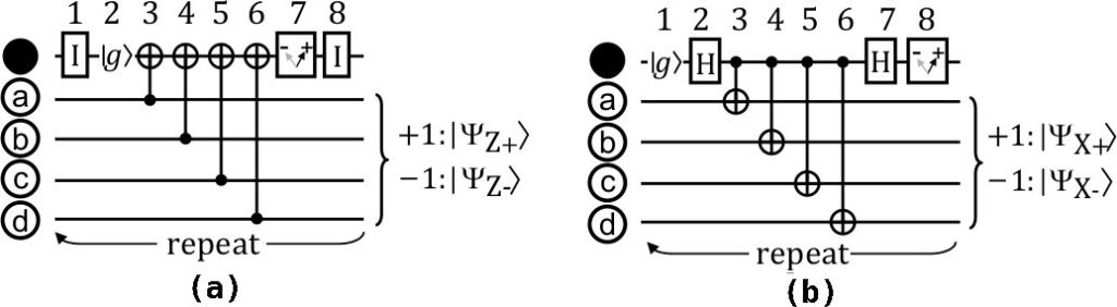
The circuit representations of the decoding corresponding to a single M–Z qubit and an M–X qubit are shown in Fig. 2. Since the same measure-qubit is shared by multiple data qubits, different errors can lead to the same syndrome in surface code. Hence the mapping from syndrome to error is not one-to-one, as illustrated in Fig. 3. This often leads to poor decoding performance by decoders. In fact, if a decoder misjudges an error e1 for some other error e2, it can so happen that e1 ⊕ e2 leads to a logical error. Therefore, not only the presence of physical errors, but also incorrect de- coding can lead to uncorrectable logical errors as well. The goal of designing a decoder, thus, is to reduce the probability of logical error for some physical error probability.
As defined in the Introduction section, the performance of a decoder is measured in terms of pseudo-threshold and threshold. With increasing code distance, the pseudo- threshold for a particular decoder also increases, which supports the intuition that using larger distance gives better protection from noise. On the other hand, the threshold does not change with respect to the distance because a de- coder for a particular surface code yields a fixed threshold. The higher are the values of these parameters, the better is the performance of the decoder. Of these two parame- ters, the pseudo threshold is lower than the threshold for a decoder. The reason is that error correction is effective be- low the pseudo-threshold point, and coding theory asserts [23] that in this region, increasing the distance of the code leads to higher suppression of logical errors. Therefore, if the threshold point is below the pseudo-threshold point it violates coding theory. Hence, it is more important for a decoder to have a higher pseudo-threshold than a higher threshold, since, beyond this error probability, QECC no longer provides any improvement in suppression of errors.
Let there be n physical qubits in a logical qubit (eg. n=d2 for surface code). A logical error can occur only when at least d of the n physical qubits are erroneous. Nevertheless, the presence of d or more physical errors does not necessarily imply the presence of a logical error. If p and pL are respectively the probability of physical and logical error, then
pL ≤ Σi pi, for d ≤ i ≤ n
Moreover, incorrect decoding itself can lead to logical errors. This can happen when the decoder fails to detect the actual physical errors and thus incorporates more errors during correction. Once again, not every incorrect decoding leads to a logical error. Therefore, if pd is the probability of failure of the decoder, then
pL ≤ Σi pi + f (pd), for d ≤ i ≤ n
where f (pd) is a function of the probability of failure of the decoder. The function f (pd) may vary with the decoder, hence the logical error probability may differ, resulting in different values of pseudo-threshold and threshold.
4. Machine learning based syndrome decoding for surface code
Machine Learning is a branch of artificial intelligence where a machine learns without being explicitly pro- grammed. Depending on the type of training data (la- beled/unlabeled/combined), the ML algorithm can vary (supervised/unsupervised/semi-supervised). It has a plethora of applications domains such as soil properties pre- diction [24], human pose estimation [25], object recognition [26], video tracking [27], prediction of the efficacy of online sale [28] etc. Here, we employ machine learning to decode error syndrome(s) for quantum error correction.
4.1. Advantages of Machine learning based syndrome decoder
Classical algorithms for decoding, such as Minimum Weight Perfect Matching (MWPM), may perform poorly in certain cases. For example, MWPM tries to find a minimum number of errors that can recreate the error syndrome obtained without considering the probability of error.
If |ψ⟩1,2,…,n is an n-qubit codeword, and we consider the error generation on this codeword is a stochastic map S (p1, p2, . . . , pn), where pi is the probability of error on qubit i (we can further write pi in terms of the probability of Pauli errors), then the error state |ψ⟩e=S (p1, p2, . . . , pn)|ψ⟩1,2,…,n. Now, for a distance d surface code with t types of errors (t=4 for depolarization, 2 for bit/phase flip), there are td2 possible errors and td2−1 possible syndromes. Therefore, multiple errors E={e1, e2, . . . , el} lead to the same syndrome, and detecting a syndrome cannot uniquely specify the type of error causing it. Since Pauli errors are hermitian, correction is simply applying the same error once more. If the choice of error is not perfect, then the system ends up with (probably) more error than before after the correction step. MWPM, being a deterministic algorithm, does not con- sider the Stochastic map. It assumes that the error probability is low, and always finds the minimum weight error emin ∈ E that creates the observed syndrome. On the other hand, an ML decoder learns the probabilities p1, p2, . . . , pn from the training phase. Thus, this decoder finds most likely error eml ∈ E that can cause observed syndrome depending on the Stochastic Map.
Furthermore, the time complexity of MWPM grows as O(N4) where N is the number of qubits. Lookup Tables have been used for decoding as well [29]. While Lookup Table Decoder is sometimes better than MWPM in performance, its complexity scales as O(4N) which becomes infeasible even for moderate values of N. To overcome such drawbacks, ML techniques have been applied to learn the probability of error in the system and propose the best possible correction accordingly with comparatively lower time complexity. For example, [19] reduced the decoding problem to a classification problem that a feed-forward neural network can solve, for small code distances. A deep neural network based decoder is proposed by [30] for Stabilizer Codes. Therefore, supervised learning techniques, such as Feed-forward neural network (FFNN), Recurrent Neural Network (RNN) show that these are capable of outperforming the traditional decoding techniques.
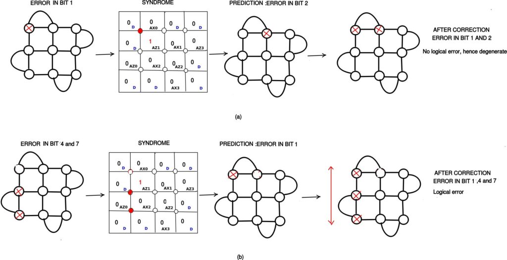
As discussed earlier, surface code is degenerate, i.e., there exist errors e1 ≠ e2 such that e1 |ψ⟩=e2 |ψ⟩, where |ψ⟩ is the codeword. This leads to any decoder failing to distinguish between some errors e1 and e2. Nevertheless, that does not always lead to a logical error. For example, bit-flip error in bit 1 and bit 2 are indistinguishable. But error in decoding these two will not lead to a logical error (Refer Fig. 4 (a)). On the other hand, it is possible that e1 ⊕ e2 leads to a logical error, i.e., the decoder may itself incorporate logical errors while correcting physical errors. For example, bit-flip error on qubit 4 is indistinguishable from those on qubits 1 and 7 together. But failure to distinguish between these two bit-flip errors leads to logical error (refer Fig. 4 (b)).
In general, usually the decoder incorporates logical errors when it fails to distinguish between ⌊(d-1)/2⌋ and ⌈(d+1)/2⌉ errors. Broadly speaking, ML can learn the probability of error and predict which of those two are more likely. This makes ML-decoder outperform other traditional decoders.
Since a decoder itself can incorporate logical errors, two stages of decoders, namely low level followed by high level
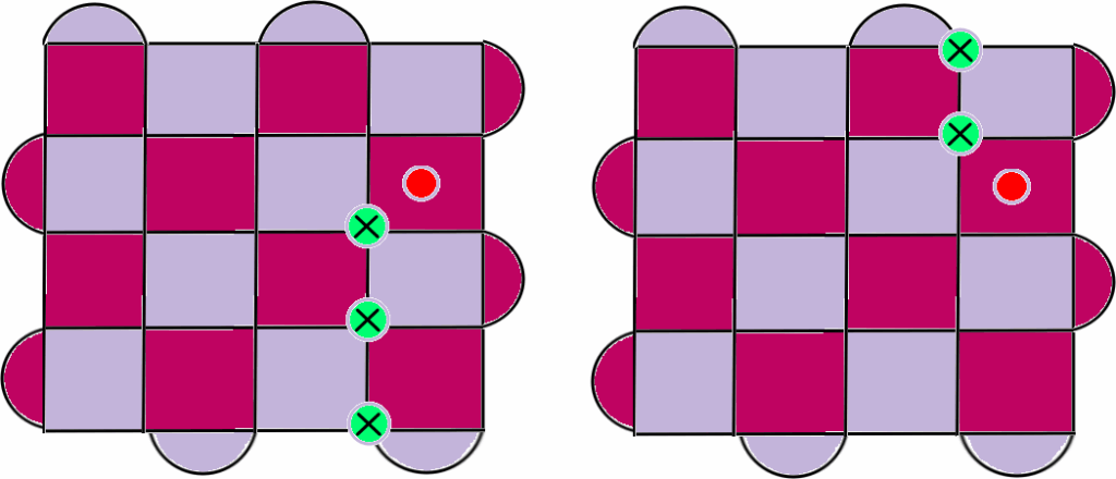
Figure 3: Example of surface code for d=5, where two errors produce the same syndrome [19]. Pink (Purple) plaquettes indicate stabilizers which check the Z (X) parity of qubits on the vertices of the plaquette. Green circles are used to indicate errors and red circles to indicate violated stabilizers.
decoder, have been applied where
- Low level decoders search for exact position of errors at the physical level.
- High level decoders attempt to correct any logical error incorporated by the correction mechanism of low level decoders.
4.1.1. Design methodology of our ML based decoder
Artificial neural networks (ANN) are made to emulate the way human brains learn, and are one of the most widely used tools in ML. Neural networks consist of one input layer, one output layer, and one or more hidden layers consisting of units that transform the input into intermediate values from which the output layer can find patterns that are too complex for a human programmer to teach the machine. The time complexity of training a neural network with N inputs, M outputs and L hidden layers is O(N · M · L). In this paper we are using neural networks as both low-level and high-level decoder for distance 3, 5, and 7 surface code.
In order to apply ML techniques to surface code decod- ing, we first map the decoding problem to the classification problem as follows. Given a set of data points, a classifica- tion algorithm predicts the class label of each data point. These techniques are purely classical. Next, we describe in detail the formulation of a decoder for surface code as a classification problem.
4.1.2. Mapping Surface Code onto a square lattice
For ease of implementation, we have mapped the surface code to a square lattice (refer Fig. 5) in this work. This has been achieved by padding a few dummy nodes (labelled as 0D in the figure). A distance d surface code is converted into a (d+1) × (d+1) square lattice which has d2 − 1 stabi- lizers, when encoding a single logical qubit. Therefore, 2(d+1) dummy nodes are required for this square lattice. The dummy nodes are basically don’t care nodes, and their value is always 0 irrespective of the error in the surface code. The syndrome changes the values of the stabilizers only.
4.1.3. Error injection and syndrome extraction
Once the distance d surface code is transformed to a (d+1) × (d+1) square lattice, the next step is to extract the syndrome for errors. First, we create a training dataset, where in each data we randomly generate errors on each physical qubit. If pphys is the probability of error on a physical qubit, the total probability of error after the 8 steps of surface code cycle (Fig. 2) is 1 – (1-pphys)8. We have trained the networks with pphys ranging from 0.0001 to 0.25. One can argue that 0.25 is an unreasonably high error probability. However, we have ranged the error probability that far to show an interesting observation regarding the ML decoder performance (Sec 4).
For generating the training data we have considered bit flip errors, symmetric and asymmetric depolarizing noise models. We have not separately considered phase flip errors since they are similar to bit flips and have a rotational symmetry (i.e., the logical errors of bit flip and phase flip model are equivalent up to a rotation by \(\frac{π}{2}\) ).
From the training data (which may or may not contain errors), we generate the syndrome (measured by ancilla qubits of the surface code) (Fig. 5). The syndrome, in our implementation, contains both the ancilla and the dummy nodes. However, the dummy nodes are always 0, whereas the values of the ancilla changes with different errors. Henceforth, in terms of implementation only, syndrome for a distance d surface code will imply (d+1)2 values including ancilla and dummy nodes. The final training data contains the syndrome, and its corresponding label is the true set of errors that have occurred in the system. Note that this method can lead to multiple labels having the same syndrome. This agrees with the fact that surface code does not have one-to-one mapping from error to syndrome.
Ideally, the dataset to achieve the best decoding performance should include all possible error syndromes. But as the code distance increases, the state space also increases exponentially. Therefore, we can at most include only a small percentage of the entire input dataset. The dataset size that we have used is 100000 from which 70000 is used for training and the rest for testing purpose.
4.1.4. Training our ML model
For the low level decoder, we train a neural network where the input layer is the syndrome and the output layer denotes the types of errors along with the physical data qubit where each error has occurred. For a distance d surface code, the number of input nodes are (d + 1)2 containing d2 – 1 measure qubits and 2(d+1) dummy nodes. For example, if we consider a distance-3 surface code (SC17), it has 8 ancilla qubits and 8 dummy nodes. Therefore, in the input layer, there are 16 nodes (Fig. 5). In the output layer, there are 2 nodes for each data qubit to differentiate among I, X, Y and Z errors. The size of the hidden layer can be adjusted by trial-and-error.
We have used two types of neural networks, (i) Feed Forward Neural Network (FFNN) and (ii) Convolutional Neural Network (CNN). In our reported results,
- FFNN consists of 2 hidden layers having 32 and 16 nodes For the cost function we have used the mean squared error rate, and as the activation function we have used Rectified Linear Unit (ReLU).
- For CNN, the first layer is a 64 dimension convolution layer where input is a 4 × 4 matrix and the kernel size is also 4 × 4. Then we flatten it and add two fully connected layers of dimension 64 and 32. After that we add the fully connected output layer of dimension 9. For the first 3 layers (convolution, dense, dense) we have used ReLu as the activation function and for the output layer we have used sigmoid activation function since it will be a multi-label classification problem.
These values were adjusted after multiple trial-and- errors. We later show in the result section that building a more complex neural network cannot provide any significant improvement in the performance of the decoder, but requires significantly more decoding time. Therefore, we stick to these parameters.
The high-level decoder simply tries to predict any logical error that has been incorporated by the low level decoder. Therefore, its input remains the same as the low-level de- coder (i.e., the syndrome) whereas it has 4 nodes in the output, each corresponding to a logical Pauli operator.
First, the network is trained for low-level decoder. After the low-level decoding is done, the predicted corrections are applied, and rechecked by using the high-level decoder whether any logical error has been inserted by the low-level decoder. The entire workflow is given in Fig. 6.
5. Results
First, we focus on the decoding performance of an ML-based low-level and the high-level decoder for surface codes of distances 3, 5, and 7 for both symmetric and asymmetric depolarizing noise models with varying degrees of asymmetry. Our model outperforms the performance of the existing decoders for symmetric noise model. We also show that although the performance of ML is slightly poorer for asymmetric noise models than that for the symmetric one, it still outperforms MWPM. Furthermore, we provide an empirical study to estimate the minimum train-test-ratio needed for optimal accuracy to obtain a better estimate of the minimum number of training data required to obtain the best (or near best) decoding results with ML decoder.
In the following subsections, we first introduce the noise model that we have considered, followed by the parameters of our ML decoder. Finally, we show the results of our decoder and compare its performance with the traditional MWPM decoder.
5.1. Noise models
Given a quantum state ρ in its density matrix formulation [5], the evolution of the state in a depolarization noise model is given as
ρ →(1 − px − py − pz)ρ+pxXρX†+pyYρY†+pZZρZ†
where px, py, pz represent the probability of occurrence of unwanted Pauli X, Y, and Z error. In symmetric depolarization noise model, px =py =pz. Moreover, quantum channels are often asymmetric or biased, i.e., the probability of occurrence of Z error is much higher than that of X or Y error. Furthermore, each error correction cycle in surface code requires eight steps. We have considered that an error can occur on one or more of the d2 data qubits in each of the eight steps, where d is the distance of the surface code. Therefore, if px + py + pz = p, then the overall probability of error for each error correction cycle is 1−(1 − p)8 (Refer Fig. 2). This error model is in accordance with [11]. We assume noise-free measure qubits (which are almost half the total number of qubits) and ideal measurements.
5.2. Machine Learning Parameters
For our study, we have trained the ML model with batches of data, not the entire data set at once. This is often beneficial in terms of training time as well as memory capacity. We have used batch size = 10000, epochs = 1000, learning rate = 0.01 (with Stochastic Gradient Descent), and we have reported the average performance of each batch over 5 instances. This is repeated for each value of the pphys considered here.
5.2.1. Low and high-level decoder
In Fig. 7, we show the increase in the logical error probability with physical error probability p, which is the probability of error per step in the surface code cycle. The results of MWPM and CNN-based low-level decoder for both symmetric and asymmetric noise models are shown. In Tables 1 and 3, we depict the performance of FFNN decoder as well. In Fig. 7, the blue, yellow, green, and red lines respectively are the decoder curves which show the probabilities of logical error for symmetric depolarization, bit flip (X), phase flip (Z), and Y errors. The cyan straight line consists of the points where the probabilities of physical and logical error are equal.
The point where the decoder curves and the straight line intersects, defines the value of pseudo-threshold for the decoder. As expected, the pseudo threshold improves with increasing distance of the surface code. Nevertheless, the threshold value is the probability of physical error beyond which increasing the distance leads to poorer performance. Therefore, threshold is independent of the distance and is a property of the surface code and the noise model only. In Tables 1 and 3, we show the pseudo-threshold and threshold of the low and high-level decoders for distance 3, 5 and 7 surface code in symmetric and asymmetric noise models respectively. Fig. 7 shows the pseudo-thresholds for MWPM and CNN decoder for a distance 3 surface code using low-level decoder (LLD) only. From Table 1 we observe ~ 10× increase in the pseudo threshold for ML-decoders as compared to MWPM.
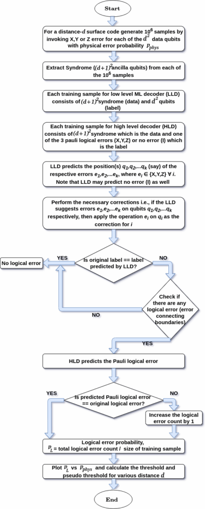
Fig. 8 shows the thresholds and decoder accuracy for MWPM and ML-decoders surface codes of distance 3, 5 and 7. Table 3 depicts the threshold values for MWPM and ML-decoders. From Table 3 we observe ∼ 2× increase in the threshold for ML-decoders as compared to MWPM.
As already mentioned earlier, this result assumes error- free stabilizers, and ideal measurements. For a distance d surface code, there are d2 − 1 stabilizers. Therefore, in our setting, nearly half of the total qubits in the surface code structure are considered ideal. We focused more on the mapping of decoding to Machine Learning in this research. A separate study is being carried out on the performance of the ML decoder in the presence of erroneous stabilizers and measure qubits to determine the threshold and pseudo-threshold. Our conjecture is that ML decoders will still outperform MWPM decoder in that scenario, but the increase in performance will be much lower.
In Fig. 7, we observe that at very low error probability the accuracy remains good, then it falls drastically. However, for ML decoders, it again increases beyond a certain physical error probability ( 0.15). On the other hand, the logical error also decreases in most of the cases for both symmetric and asymmetric ML decoders after more or less that same value of physical error probability. This is due to the bias in the back-end working principle of any machine learning model. When the error probability is low or high, the ML decoder effectively learns the probability and in most of the cases can avoid logical errors. But when the error probability is in the mid range, the ML model gets confused. For example, if in a training set, out of 12 events with same value of the features, 10 events are certainly in class A, and the rest in B, then the ML definitely learns it with high accuracy. Similarly, if those same 10 events are in class B, accuracy will be high. But the ML is confused when 6 of them are in class A and 6 of them in class B. This is an interesting observation in the ML-decoder which is absent in MWPM-decoder.
5.3. More sophisticated ML models
A natural question is whether the use of more sophisticated ML models (e.g, adding more hidden layers, increasing the number of nodes in each layer, etc.) can improve the performance of the decoder. We have addressed this issue as reported below.
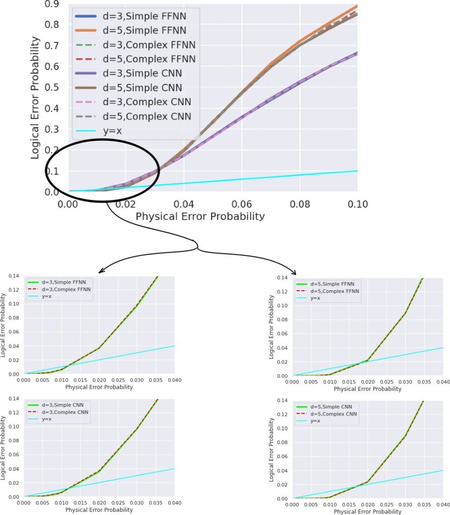
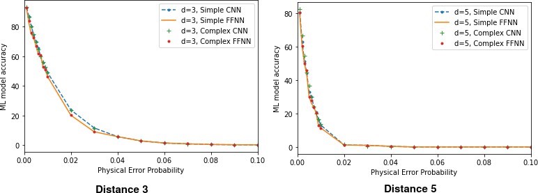
In Table 2, Simple FFNN has 1 hidden layer (dense) whereas Complex FFNN has 5 hidden layers (dense) and Simple CNN has 1 convolution (64 dimensions) followed by 2 dense layers of dimension 256 and 64 respectively before the output layer whereas Complex CNN has 3 convolutions (64 dimensions) layers followed by 4 dense layers of dimension 512, 256, 128 and 64 respectively before the output layer. The more sophisticated models naturally require more time for training and prediction. But from Fig. 9, we see that the decoder graphs are more or less overlapping for the simple and complex ML models. Therefore, it can be concluded that using more sophisticated model does not lead to a better performance for the decoder. This can be further verified by the accuracy plots in Fig. 10. Since the more complex models are performing almost at par with the simpler models for d=3 and 5 and the complex models are significantly more time-consuming, we performed the experiments for d = 7
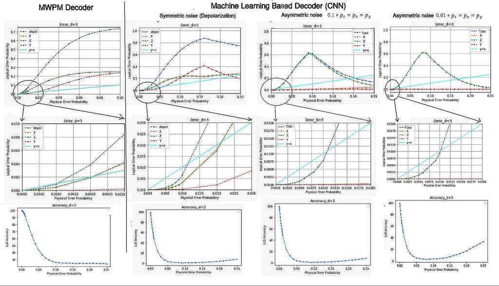
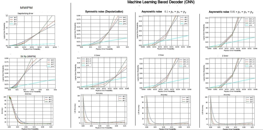
Table 1: Pseudo-Threshold of the low and high level decoders for distance 3, 5 and 7 surface code
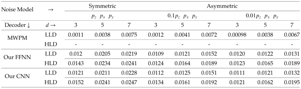
Table 2: Comparison of training times for different ML models
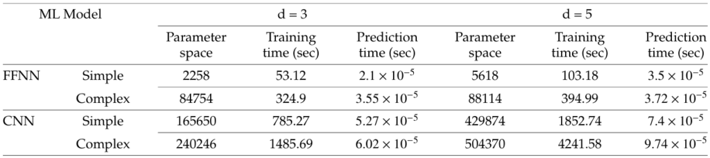
Table 3: Comparison of Threshold of the low and high level decoders
Threshold (LLD) | Threshold (HLD) | Decoder Model | Error model |
0.0181 | N/A | MWPM | Symmetric |
0.0302 0.0218 0.0221 0.0216 0.0213 | 0.035 0.025 0.0279 0.0257 0.0251 | Our FFNN | Symmetric Asymmetric 0.1 ∗ pz = px = py Asymmetric 0.07 ∗ pz =px = py Asymmetric 0.04 ∗ pz=px= py Asymmetric 0.01 ∗ pz =px=py |
0.0311 0.0225 0.0229 0.0223 0.0212 | 0.034 0.026 0.0281 0.0258 0.0252 | Our CNN | Symmetric Asymmetric 0.1 ∗ pz=px =py Asymmetric 0.07 ∗ pz=px= py Asymmetric 0.04 ∗ pz= px= py Asymmetric 0.01 ∗ pz= px= py |
with only Simple CNN and FFNN models.
5.4. Empirical train-test-ratio for optimal accuracy
In general, the higher the number of training samples, better is the accuracy of the ML model up to a certain threshold, be- yond which increasing the number of training samples does not improve the performance of the model [31]. However, generation of training data is a humongous task in current quantum devices since it takes up a significant amount of device lifetime. Therefore, lower the size of the training sample required, higher is its usability. But naively reducing the size of the training set may lead to performance degradation. We explore this requirement by studying the minimum train-test-ratio required to obtain the optimal decoder performance.
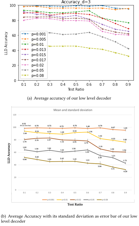
Given a distance d code, with t types of errors possible on each qubit, the total number of distinct error patterns is td2. When the probability of error is very low, most of the test cases will have no error. This observation is reflected in the curve [Fig 11] with p = 0.001. As p increases, it is natural that the performance of the decoder will degrade. However, when d is small, the total number of distinct errors is also small. Since the training and testing data is generated uniformly at random, we expect that for a given error probability p, the most likely error patterns are all exposed to the ML decoder for a reasonable size of training set.
To test this hypothesis, in Fig. 11 we have varied the train-test ratio for the simple CNN decoder for a distance 3 surface code. We originally generated 105 error data uniformly at random, and varied the train-test ratio starting from 90:10 and moving up to 10:90, lowering the training proportion by 10% in each step. The obtained accuracy for increasing pphys is plotted in Fig. 11. We observe that even when we use up ≃ 50 − 60% of the data as test set, the performance of the decoder remains more or less constant for a given p. The performance takes a dip downwards beyond this value. Therefore, we posit that for d = 3 and t = 4 (depolarizing noise model), this decoder is exposed to all of the most likely errors within a small fraction of the training set, which is generated uniformly at random.
Since this is a ML based method, and Fig. 11(a) shows the mean value only, in Fig. 11(b) we have also plotted the standard deviation (SD) with a few values of physical error probability for all the test-ratio as an error bar plot. We observe that for p=0.001 the accuracy varies between 95.32 to 99.11 (min SD = 0.52, max SD = 1.40). For p = 0.02 the accuracy varies between 60.54 to 82.94 (min SD = 1.12, max SD = 2.79) and for p = 0.08 the accuracy varies between 32.51 to 51.92 (min SD = 0.28, max SD = 3.86). With increasing pphys, the SD also increases. This supports intuition because as the pphys increases, the decoding performance decreases due to the capacity of the machine learning model to correctly classify the errors. Hence, the performance of ML (which depends on the errors in the dataset), varies more with higher value of physical error probability (pphys).
Moreover, as d increases, for same p, the set of probable errors increases exponentially. Therefore, for the same number of generated error data, we expect that to retain the same accuracy, a much larger portion of the data will need to be devoted for training. In our future research, we shall explore this direction in a more extensive manner and determine the size of the training sample required to retain an accuracy ϵ for a given train-test ratio.
5.5. Performance on Training with Symmetric Noise Models and Testing with Asymmetric Noise Models
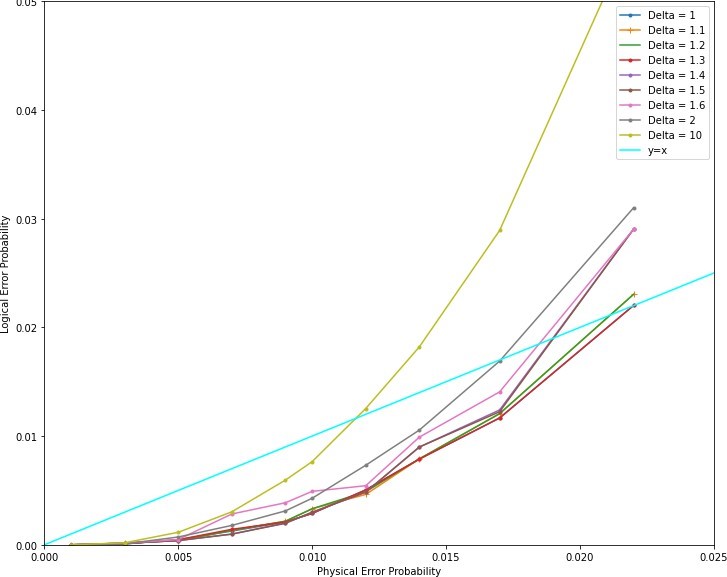
As we have discussed, the real life noise models are asymmetric. But this asymmetry can change and we may not know the exact level of asymmetry beforehand always. It would be beneficial if the decoder can be trained once with symmetric noise dataset and tested with different asymmetric noise datasets. Now we analyze how the performance of a decoder trained with symmetric noise model behaves while testing with asymmetric noise model with increase in asymmetry (∆).
An increase in asymmetry (∆) in the depolarizing error channel is denoted by px = p/(∆+2), py = p/(∆+2), pz = p∆/(∆+2), where, p is the value of physical error rate for a given physical error. For example, ∆ = 10 denotes 0.1 ∗ pz=px =py. For symmetric noise model, ∆ = 1 and for asymmetric noise model, ∆ > 1. We define crossover point to be the value of ∆ beyond which increasing ∆ leads to lower pseudo- threshold, when the decoder is trained with symmetric noise. We say that the channel is weakly asymmetric if ∆ < cross-over point, strongly asymmetric otherwise. And we find the crossover point empirically.
As the asymmetry increases in the testing data, step- wise, we see a decrease in the performance of the decoder, as inferred from their decreased pseudo-threshold values. We check for ∆=1, 1.1, 1.2, 1.3, 1.4, 1.5, 1.6, 2, 10.
From Fig. 12 we can say that ∆ = 1.3 is the crossover point as upto this point, the logical error more or less overlaps with the symmetric noise model (i.e. ∆=1). Hence upto ∆ = 1.3, the channel is weakly asymmetric and above ∆ = 1.3 it is strongly asymmetric. Hence, upto ∆ = 1.3 we can train the decoder with symmetric noise model and test with the desired symmetric or asymmetric noise model, as it will not degrade the performance much. However, beyond this degree of asymmetry, the model must be trained with the asymmetric noise model if the optimum pseudo-threshold is to be obtained.
6. Conclusion
In this paper, we have proposed an ML-decoder to correct both symmetric and asymmetric depolarizing noise on sur- face codes. Our decoder has two levels — in the low-level it tries to accurately predict the error on the qubits, followed by the high level that tries to detect any logical error that
may have been introduced by the low-level decoder. Both these decoders have been implemented using neural net- work (FFNN and CNN) for surface code of distances 3, 5 and
- Our proposed ML-decoder outperforms MWPM, and we observe ∼ 2× increase in threshold and ∼ 10× increase in pseudo threshold. We further show that the decoder performance is equally good for asymmetric errors as well, which is more realistic in quantum devices.
We have used ML models with different levels of sophistication, (i.e. varying number of hidden layers and node-density of each layer). Our results show that the mere increase of complexity in ML model requires an increased amount of time for decoding but hardly yields any better performance.
In this work, we have assumed, noise-free measure qubits and ideal measurements. A future prospect of this research can be to consider noisy measure qubits and imperfect measurements.
Data and Code availability
Data from the numerical simulations and the code can be made available upon reasonable request.
Conflict of Interest The authors declare no conflict of interest.
- P. W. Shor, “Polynomial-time algorithms for prime factorization and discrete logarithms on a quantum computer”, SIAM J. Comput., vol. 26, no. 5, pp. 1484–1509, 1997, doi:10.1137/S0097539795293172.
- L. K. Grover, “A fast quantum mechanical algorithm for database search”, “Proceedings of the Twenty-eighth Annual ACM Symposium on Theory of Computing”, STOC ’96, pp. 212–219, ACM, New York, NY, USA, 1996, doi:10.1145/237814.237866.
- A. M. Childs, N. Wiebe, “Hamiltonian simulation using linear com- unitary operations”, Quantum Info. Comput., vol. 12, no.
12, p. 901–924, 2012. - J. R. McClean, J. Romero, R. Babbush, A. Aspuru-Guzik, “The theory of variational hybrid quantum-classical algorithms”, New Journal of Physics, vol. 18, no. 2, p. 023023, 2016.
- M. A. Nielsen, I. Chuang, Quantum computation and quantum informa- tion, AAPT, 2002.
- P. W. Shor, “Scheme for reducing decoherence in quantum com- puter memory”, Phys. Rev. A, vol. 52, pp. R2493–R2496, 1995, doi: 10.1103/PhysRevA.52.R2493.
- A. M. Steane, “Error correcting codes in quantum theory”, Phys. Rev. Lett., vol. 77, pp. 793–797, 1996, doi:10.1103/PhysRevLett.77.793.
- R. Laflamme, C. Miquel, J. P. Paz, W. H. Zurek, “Perfect quantum error correcting code”, Phys. Rev. Lett., vol. 77, pp. 198–201, 1996, doi:10.1103/PhysRevLett.77.198.
- S. B. Bravyi, A. Y. Kitaev, “Quantum codes on a lattice with boundary”,
arXiv preprint quant-ph/9811052, 1998. - E. Dennis, A. Kitaev, A. Landahl, J. Preskill, “Topological quantum memory”, Journal of Mathematical Physics, vol. 43, no. 9, pp. 4452–4505, 2002.
- A. G. Fowler, A. M. Stephens, P. Groszkowski, “High-threshold uni- versal quantum computation on the surface code”, Physical Review A, vol. 80, no. 5, p. 052312, 2009.
- D. S. Wang, A. G. Fowler, L. C. Hollenberg, “Surface code quantum computing with error rates over 1%”, Physical Review A, vol. 83, no. 2, p. 020302, 2011.
- L. Riesebos, X. Fu, S. Varsamopoulos, C. G. Almudever, K. Bertels, “Pauli frames for quantum computer architectures”, “Proceedings of the 54th Annual Design Automation Conference 2017”, pp. 1–6, 2017.
- A. G. Fowler, A. C. Whiteside, L. C. Hollenberg, “Towards practical classical processing for the surface code”, Physical review letters, vol. 108, no. 18, p. 180501, 2012.
- R. Majumdar, S. Basu, P. Mukhopadhyay, S. Sur-Kolay, “Error trac- ing in linear and concatenated quantum circuits”, arXiv preprint arXiv:1612.08044, 2016.
- J. Edmonds, “Paths, trees, and flowers”, Canadian Journal of Mathemat- ics, vol. 17, p. 449–467, 1965, doi:10.4153/CJM-1965-045-4.
- S. Varsamopoulos, K. Bertels, C. G. Almudever, “Comparing neural network based decoders for the surface code”, IEEE Transactions on Computers, vol. 69, no. 2, pp. 300–311, 2019.
- C. Chamberland, P. Ronagh, “Deep neural decoders for near term fault-tolerant experiments”, Quantum Science and Technology, vol. 3, no. 4, p. 044002, 2018.
- S. Varsamopoulos, B. Criger, K. Bertels, “Decoding small surface codes with feedforward neural networks”, Quantum Science and Technology, vol. 3, no. 1, p. 015004, 2017.
- R. Sweke, M. S. Kesselring, E. P. van Nieuwenburg, J. Eisert, “Rein- forcement learning decoders for fault-tolerant quantum computation”, Machine Learning: Science and Technology, vol. 2, no. 2, p. 025005, 2020.
- L. Ioffe, M. Mézard, “Asymmetric quantum error-correcting codes”,
Phys. Rev. A, vol. 75, p. 032345, 2007, doi:10.1103/PhysRevA.75.032345. - D. Gottesman, “Stabilizer codes and quantum error correction”, arXiv preprint quant-ph/9705052, 1997.
- R. Hill, A first course in coding theory, Oxford University Press, 1986.
- V. Kumar, J. S. Malhotra, S. Sharma, P. Bhardwaj, “Soil Properties Pre- diction for Agriculture using Machine Learning Techniques”, Journal of Engineering Research and Sciences, vol. 1, no. 3, pp. 9–18, 2022.
- H.-Y. Tran, T.-M. Bui, T.-L. Pham, V.-H. Le, “An Evaluation of 2D Human Pose Estimation based on ResNet Back-”, Journal of Engineering Research and Sciences, vol. 1, no. 3, pp. 59–67, 2022.
- M. A. Danlami, A. O. Oluwaseun, M. S. Adam, S. M. Abubakar, E. Ay- obami, “Cascaded Keypoint Detection and Description for Object on”, Journal of Engineering Research and Sciences, vol. 1, no. 3,
. 164–169, 2022. - S. K. Pal, D. Bhoumik, D. Bhunia Chakraborty, “Granulated deep learning and z-numbers in motion detection and object recognition”, Neural Computing and Applications, vol. 32, no. 21, pp. 16533–16548, 2020.
- A. V. Singhania, S. L. Mukherjee, R. Majumdar, A. Mehta, P. Banerjee,
D. Bhoumik, “A machine learning based heuristic to predict the ef- ficacy of online sale”, “Emerging Technologies in Data Mining and Information Security”, pp. 439–447, Springer, 2021. - S. Varsamopoulos, K. Bertels, C. G. Almudever, “Designing neu- ral network based decoders for surface codes”, arXiv preprint arXiv:1811.12456, 2018.
- S. Krastanov, L. Jiang, “Deep neural network probabilistic decoder for stabilizer codes”, Scientific reports, vol. 7, no. 1, pp. 1–7, 2017.
- vid, Understanding machine learning: From algorithms, Cambridge university press, 2014.
No related articles were found.