A product’s life cycle hinges on its sales. Product sales are determined by a combination of market demand, industrial production, logistics, supply chains, labor hours, and countless other factors. Business-specific questions about sales are often formalized into questions relating to specific quantities in sales data. Statistical estimation of these quantities of interest is crucial but restricted availability of empirical data reduces the accuracy of such estimation. For example, under certain regularity conditions the variance of maximum likelihood estimators cannot be asymptotically lower than the Cramer-Rao lower bound. The presence of additional information from external sources therefore allows the improvement of statistical estimation. Two types of additional information are considered in this work: unbiased and possibly biased. In order to incorporate these two types of additional information in statistical estimation, this manuscript minimizes mean squared error and variance. Publicly available Walmart sales data from 45 stores across 2010-2012 is used to illustrate how these statistical methods can be applied to use additional information for estimating weekly sales. The holiday effect (sales spikes during holiday weeks) adjusted for overtime trends is estimated with the use of relevant external information.

1. Introduction

Sales data is highly important in a product’s life cycle. Sales data is the place where the market demand and industrial supply meet and balance each other to impact inventory management, logistics, supply chains, and more. There are many business-specific questions sales data help address. Typically, these questions are formalized into quantities determined by sales data. Business owners may be interested in the impact of an advertisement campaign, the effect of a holiday on sales, or seasonal trends. Since sales data widely fluctuate, these quantities are considered to be random variables.

The behaviours of these random quantities (i.e. random variables) are described by their probability distributions, estimated with previously collected observations. In [1], the author uses sales data and considers exponential and normal models to reduce the Total Operating Cost. In [2], the authors combine online reviews and historic sales data to forecast sales. In [3], the authors suggest to maximize the direct profit based on both maximization of profit and parameter estimation.

Many of these statistical methods rely on regular estimators– the estimators which have two finite moments. This means that the central limit theorem is applicable, and external information (e.g., averaged sales) known with some uncertainty (e.g., variance) can be incorporated in the statistical estimation procedure to improve accuracy. In [4], Tarima and Pavlov propose a method for incorporating uncertain external information in statistical estimation. [4] and [5] postulate the unbiasedness of additional information. This, for example, means that in different stores the expected sales are the same. [6] derived asymptotic relative efficiency of the estimators proposed in [4]. Previously published data were used in statistical estimation in [7].

It is possible that the external information may estimate a different quantity, leading to a biased external estimate of a quantity of interest. To account for such bias, mean squared error (MSE) is minimized instead in [8, 9]. External information given in the form of a set of possible values is used in [10]–[11], MSE is also minimized. In [12], the author used additional quantile information.

This manuscript shows how external information on sales can be used under (1) the assumption that the external information came from an unbiased data source and (2) that the external data source can be very different to assume unbiasedness. This manuscript is an updated and extended version of a proceedings paper [13] where similar statistical methodology was applied to newsvendor-type problems. Section 3 presents main mathematical results for combining empirical and external data summarized by sample means and their variances. Sections 2 and 4 use these statistical methods for estimating the adjusted holiday effect using publicly available weekly sales data for Walmart stores in 2010-2012. The example was implemented in R [14], see Appendix for the relevant R code.

Table 1: Parameters and their estimators; E denotes mathematical

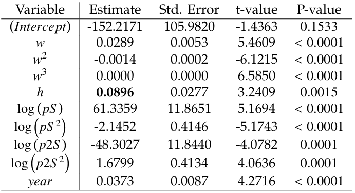
Table 2: Table of regression coefficients for modelling log (weekly sales) [“store id” = 1]; w is a week, h is a holiday indicator, pS is a previous weekly sales, and p2S is the sales from two weeks ago.

2. Illustrative Example

Walmart weekly sales data for a sample of 45 Walmart stores over the period of 2010-2012 became available to public via a Kaggle competition (www.kaggle.com). This dataset was later used by researchers and data scientists for research and educational purposes, see [15]–[16].

For illustrative purposes, the dataset is reduced down to four variables:

• “Store ID”: 1 though 45,
• “Date”: a week of sales (48 weeks in 2010, 52 weeks in 2011 and 43 weeks in 2012)
• “Sales”: total weekly sales, and
• “Holiday”: a holiday

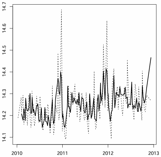
To illustrate the overtime pattern associated with sales within this dataset, a linear autoregressive model was fitted to model weekly sales on a logarithmic scale using the first store data (“store id” = 1). The model’s table of regression coefficients is shown in Table 2.

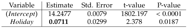
Consider the objective of estimating a holiday effect controlling for the overtime sales pattern. The overtime sales pattern controls for the yearly linear effect, the cubic approximation yearly seasonality, and the quadratic approximation of sales within the two previous weeks. The holiday effect adjusted for this overtime pattern is estimated by the regression coefficient and is equal to 0.0896 for store #1. Since the modelling is completed on the logarithmic scale, the effect on total sales is multiplicative and is equal to 1.0937 = exp 0.0896 , meaning that controlling for the over-time trend ≈9.4% increase in total sales is anticipated. This is the adjusted effect, which is different from the unadjusted holiday effect. The unadjusted effect, in our definition, is a proportional increase during holiday weeks as compared to non-holiday weeks. This effect can be estimated by a simple linear regression model reported in Table 3: the unadjusted effect is expressed by the regression coefficient 0.0711, leading to an unadjusted increase in sales ≈7.4% (exp 0.0711 =1.0737).

Table 3: Table of regression coefficients for modelling log(weekly sales) [“store id” = 1]; simple linear regression, unadjusted analysis.

Let’s assume that a researcher is able to get access to nine stores and perform the same adjusted and unadjusted analyses for each of the stores: see Table 4 for the results.

Table 4: Adjusted and unadjusted regression coefficients of the holiday effect for the nine stores.

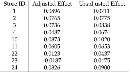
The nine observed adjusted holiday effects can be used to estimate the expected holiday effect (θ) adjusted for the overtime trend. This effect, θ, is not conditional on a specific store but averaged across all stores. The estimate of θ,ˆθ=0.0569 and an estimate of its variance is 0.000154.

Suppose that unadjusted holiday effects are also avail- able for the rest of the stores. The researcher classifies the stores into two groups. One group of stores aggregates stores with similar characteristics, and it is expected that the impact of holidays on sales numbers is the same, see Table 5. Other stores are different and it is possible that the holiday effect is different too, See Table 6.

Table 5: Unadjusted regression coefficients of the holiday effect available for the 25 stores with correlated sales.

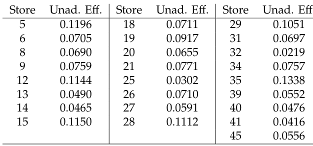
Table 6: Unadjusted regression coefficients of the holiday effect available for the 11 stores with uncorrelated sales.

Can these two external sources of information be used to improve estimation accuracy of the the adjusted holiday effect? The answer is yes, and we will return to this illustrative example later in Section 4.

3. Methodology

This section presents the main statistical formulas regarding the use of external information proposed in [4, 5] (variance minimization), and [8, 17] (MSE minimization) and applies these methods to Walmart sales data.

3.1. Parameters and their Estimators

Let θ be a parameter of interest. In Section 2, the quantity of interest is

$$\theta = E\left(\log(S) \mid w = w,\, pS = l_1,\, p2S = l_2,\, h = 1\right) – E\left(\log(S) \mid w = w,\, pS = l_1,\, p2S = l_2,\, h = 0\right), \tag{1}$$

where the terms are explained in Table 2. An estimator of θ based on the nine Walmart stores from Table 4 is assumed to have no bias, E ˆθ =θ. Another estimator ~η, known as external information, estimates η, which can be different from θ. In Section 2,

$$\eta = E\left(\log(S) \mid h = 1\right) – E\left(\log(S) \mid h = 0\right), \tag{2}$$

is the unadjusted holiday effect. Since the data in Table 6 correspond to a different cohort of stores, the unadjusted holiday effect estimated on data from Table 6 may be a biased estimate of η (the stores from Table 6 may not be- long to the population of interest). Additional external information from Tables 5 and 6 can be converted into a two-dimensional estimate \(\tilde{\eta} = (\tilde{\eta}_1, \tilde{\eta}_2) = (0.0737, 0.0261)\) The number 0.0737 is an unbiased estimate of \(\eta,\, E(\tilde{\eta}_1) = \eta\) Note that Table 4 can also be used to estimate η, because the unadjusted holiday effect was also estimated for each of the nine stores, \(\hat{\eta}_1 = 0.0720\) The second number in \(\tilde{\eta} \, (\tilde{\eta}_2 = 0.0261)\) is a possibly biased estimate of \(\eta,\, E(\tilde{\eta}_2) = \eta + \delta\)

Further, we use a “hat” to denote estimators based on the main dataset and a “tilde” for additional information quantities.

3.2. Method

To combine external information with the main data, we use the family of estimators:

$$\theta^{\Lambda} = \hat{\theta} + \Lambda \left( \tilde{\eta} – \bar{\eta} \right), \tag{3}$$

where Λ is an unknown (possibly multidimensional) parameter. In (3), \(\hat{\eta}\) is an estimate based on the main data. Note that \(E(\tilde{\eta}) = \eta\) but \(E(\tilde{\eta}) = \eta + \delta\) where δ is a possible bias or a vector of biases. Section 2 bias has two components and

$$\hat{\delta} = \hat{\eta} – \tilde{\eta} = (0.0720, 0.0720) – (0.0737, 0.0261) = (-0.0017, 0.0459). \tag{4}$$

Following [8], minimum MSE among  θ^Λ estimators is reached at

$$\theta^{0}(\delta) = \hat{\theta} – \mathrm{cov}(\tilde{\theta}, \tilde{\delta}) \, E^{-1}(\tilde{\delta} \tilde{\delta}^T) \, \tilde{\delta}^T \tag{5}$$

and

$$MSE(\theta^0) = \mathrm{cov}(\hat{\theta}) – \mathrm{cov}(\hat{\theta}, \tilde{\delta}) \, E^{-1}(\tilde{\delta} \tilde{\delta}^T) \, \mathrm{cov}(\tilde{\delta}, \hat{\theta}),$$

where \(E(\tilde{\delta} \tilde{\delta}^T) = \mathrm{cov}(\hat{\eta}) + \mathrm{cov}(\tilde{\eta}) + \delta \delta^T \quad \text{and “}\mathrm{cov}(\cdot)\text{”}\) is a variance-covariance matrix.

The special case of δ=0 makes θ^Λ unbiased. Then,

$$\theta^{0}(0) = \hat{\theta} – \mathrm{cov}(\hat{\theta}, \hat{\delta}) \, \mathrm{cov}^{-1}(\hat{\delta}) \, \hat{\delta}^T \tag{6}$$

achieves minimal variance in θ^Λ, see [4]; T denotes transposition. Then

$$\mathrm{cov}(\theta^{0}(0)) = \mathrm{cov}(\hat{\theta}) – \mathrm{cov}(\hat{\theta}, \hat{\delta}) \, \mathrm{cov}^{-1}(\hat{\delta}) \, \mathrm{cov}(\hat{\delta}, \hat{\theta}) \tag{7}$$

For a one-dimensional case, the quadratic form in Equation (7) is

$$M = \mathrm{cov}(\hat{\theta}, \hat{\delta}) \, \mathrm{cov}^{-1}(\hat{\delta}) \, \mathrm{cov}(\hat{\delta}, \hat{\theta}) \geq 0$$

• If ˆθ and ˆδ are uncorrelated, \(M = 0 \text{ and } \theta^0(\delta) = \hat{\theta} \,\, \forall \, \tilde{\eta}.
  \)
• \(\text{If } \mathrm{cov}(\hat{\theta}, \tilde{\delta}) = \mathrm{cov}(\hat{\theta}) \ (\eta = \theta),\quad M = \mathrm{cov}(\hat{\theta}),\quad \theta^0(0) = \theta \text{ and } \mathrm{cov}(\theta^0(0)) = 0.\)

The estimator θ⁰ (δ) needs covariances to be applicable in practice. Plus, δ is also unknown. Dmitriev and his colleagues [10] used the same family of estimators. They assumed \(\tilde{\eta} = \eta + \delta,\) belongs to a pre-determined set of values.

We use the main data to estimate unknown quantities in θ⁰ (δ) :

$$\hat{\theta}^0(\delta) = \hat{\theta} – \widehat{\mathrm{cov}}(\hat{\theta}, \tilde{\delta}) \left( \widehat{\mathrm{cov}}(\hat{\eta}) + \widehat{\mathrm{cov}}(\tilde{\eta}) + \delta \delta^T \right)^{-1} \tilde{\delta}^T. \tag{8}$$

3.3. Large sample properties

Let θ and η be scalar quantities. Under certain regularity conditions

$$\sqrt{n} \left( \hat{\theta}^0(\delta) – \theta^0(\delta) \right) = o_p(1). \tag{9}$$

Consequently, ∀ fixed δ ≠ 0,

$$\sqrt{n} \left( \theta^0(\delta) – \theta \right) = o_p(1). \tag{10}$$

and

$$\sqrt{n} \left( \widehat{\theta}^0(\delta) – \theta \right) = o_p(1). \tag{11}$$

From (10) and (11)

$$\sqrt{n} \left( \hat{\theta}^0(\delta) – \theta^0(\delta) \right) = o_p(1). \tag{12}$$

Estimator ˆθ⁰ (δ) still cannot be used in practice because δ is know known. The use ˆδ leads to

$$\hat{\theta}^0(\delta) = \hat{\theta} – \widehat{cov}(\hat{\theta}, \hat{\delta}) \left( \widehat{cov}(\hat{\eta}) + \widetilde{cov}(\tilde{\eta}) + \hat{\delta} \hat{\delta}^T \right)^{-1} \hat{\delta}^T. \tag{13}$$

The application of ˆδ instead of δ makes (9) in valid: if \(\delta = 0, \quad \sqrt{n} \left( \hat{\theta}^0(\hat{\delta}) – \theta^0(0) \right) = O_p(1)\) which means that \(\sqrt{n} \left( \hat{\theta}^0(\hat{\delta}) – \theta^0(0) \right)\) does not go to zero, in probability.

Let \(\delta = \delta_1 \sqrt{n},\) whereδ₁ ∈ (−∞,+∞) is a local alternative, n denote the sample size of the empirical data set available to the data analyst, and m be the size of the dataset used to obtain additional information. For the analysis of asymptotic properties we will tie these two sample sizes asymptotically with \(\frac{n}{m} \rightarrow k\), where k is a non-negative real number or a  +∞. We assume that the estimators based on empirical and  external data are regular enough so that the law of large numbers applies:

$$K_{\theta, \eta} = \lim_{n \to \infty} n \cdot \widehat{cov}(\widehat{\theta}, \widehat{\delta}) = \lim_{n \to \infty} n \cdot \widehat{cov}(\widehat{\theta}, \widehat{\eta}),$$

$$K_{\eta, \eta} = \lim_{n \to \infty} n \cdot \widehat{cov}(\widehat{\eta}),$$

$$K_{\theta, \theta} = \lim_{n \to \infty} n \cdot \widehat{cov}(\widehat{\theta}),$$

and

$$K’_{\eta, \eta} = \lim_{m \to \infty} m \cdot \widetilde{cov}(\widetilde{\eta})$$

are constants (asymptotic covariances). We will also assume that a central limit theorem applies so that

$$\xi_{\theta} = N(0, K_{\theta, \theta}) = \lim_{n \to \infty} \sqrt{n} \left( \widehat{\theta} – \theta \right),$$

$$\xi_{\eta} = N(0, K_{\eta, \eta}) = \lim_{n \to \infty} \sqrt{n} \left( \widehat{\eta} – \eta \right),$$

$$\xi’_{\eta} = N(0, K’_{\eta, \eta}) = \lim_{m \to \infty} \sqrt{m} \left( \widetilde{\eta} – \eta \right),$$

and, consequently,

$$\xi_{\delta} = \lim_{n \to \infty} \sqrt{n} \left( \widehat{\delta} – \delta \right)$$

$$= \lim_{n \to \infty} \sqrt{n} \left( \widehat{\eta} – \eta \right)$$

$$- \sqrt{k} \lim_{m \to \infty} \sqrt{m} \left( \widetilde{\eta} – \eta – \delta_1 \sqrt{m} \right)$$

$$= N\left( \delta_1, K_{\eta, \eta} + k K’_{\eta, \eta} \right).\tag{14}$$

The  random  variable  ξ_δ  can  be  represented  as \(\xi_{\delta} = \xi_{\eta} + \sqrt{k} \xi_{\eta’},
\) which shows that ξ_δ and ξ_θ can be correlated because ξ_θ and ξ_η are based on the same dataset. 

Thus, the asymptotic behaviour of \(\widehat{\theta}^{0}(\tilde{\delta})\) differs from a normal distribution. Then the non-normal asymptotic behavior for large samples is

$$\sqrt{n} \left( \theta^0(\tilde{\delta}) – \theta \right) = \sqrt{n} \left( \widehat{\theta} – \theta \right)$$

$$- \, n \cdot \widehat{cov}(\theta, \delta) \left[ n \cdot \widehat{cov}(\eta) \right]$$

$$+ \left[ n \cdot \widetilde{cov}(\eta) + n \cdot \widetilde{\delta \delta^T} \right]^{-1} \sqrt{n} \cdot \widehat{\delta}$$

$$\xrightarrow{d} \xi_\theta – K_{\theta,\eta} \left( K_{\eta,\eta} + k K’_{\eta,\eta} + \xi_\delta^2 \right)^{-1} \xi_\delta.\tag{15}$$

The above asymptotic behaviour depends on two (de- pendent) normal random variables \(\xi_\delta \left(= \sqrt{n} \left( \widehat{\theta} – \theta \right) \right)\) and \(\xi_\theta \left(= \sqrt{n} \cdot \widehat{\delta} \right)\).

Overall, if δ = 0 can be surely assumed, the minimum variance estimator \(\widehat{\theta}^{0} (0)\) is to be used, and if some protection against possible bias (disinformation/misinformation) is needed then minimum MSE estimation with \(\widehat{\theta}^{0} (\tilde{\delta})\) is a better choice with the understanding that \(\widehat{\theta}^{0} (\tilde{\delta})\) is inferior to \(\widehat{\theta}^{0} (0)\) under δ=0. The large sample distribution of \(\widehat{\theta}^{0} (\tilde{\delta})\) differs from normal, but is known, see (15). The estimator \(\widehat{\theta}^{0} (\tilde{\delta})\) an be used to evaluate the impact of bias on the estimating procedure.

3.4. A Monte-Carlo simulation study comparing minimum variance and minimum MSE estimation

To illustrate large sample properties of minimum variance and minimum MSE approaches, we have performed a Monte-Carlo experiment with 500, 000 repetitions. The statistical model generated two samples: (1) the empirical sample, which is a sample with 100 paired standard normal random variables (X₁ and Y₁) with cor .X₁, Y₁ =0.9 and (2) the external sample with 1000 standard normal random variables (X₂). The objective is to estimate the mean of Y, which is equal to zero in this example.

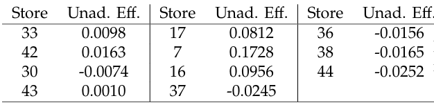
The asymptotic distribution of \(\hat{\theta}\) (mean of Y₁) is approximately normal, so that \(\sqrt{100} \cdot \hat{\theta}\) ∼ N (0, 1) leading to the width of 95% for \(\sqrt{100} \cdot \hat{\theta}\) equal to 3.92 (=2 · 1.96). The asymptotic distribution of \(\sqrt{100} \cdot \hat{\theta}^{0}(0)\) is also approximately normal with mean =0 and variance =0.266358, see Figure 2. The distance between 2.5% and 97.5% level quantiles of the distribution of \(\sqrt{100} \cdot \hat{\theta}^{0}(0)\) is equal to 2.03227. Wald’s confidence interval (“mean estimate” ±1.96 “standard deviation of the estimate”) had an almost identical length (=2.023107).
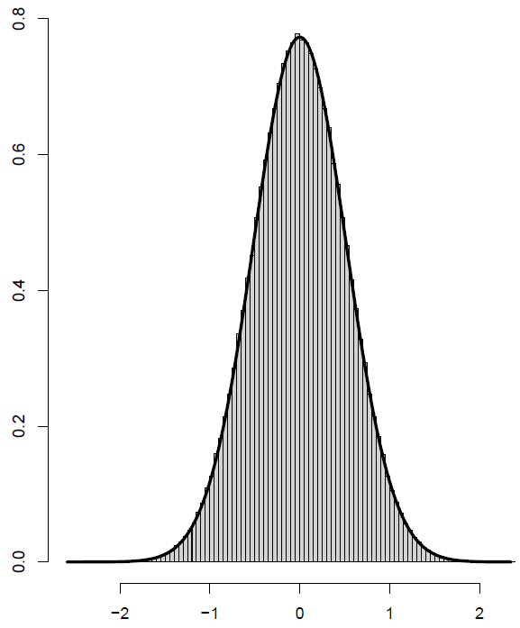
The asymptotic distribution of \(\sqrt{100} \cdot \widehat{\theta^0} \left( \widehat{\delta} \right)\) is not normal anymore and is shown in Figure 3. The normal approximation allows us to visually evaluate the departure from normality. The absence of asymptotic normality, however, is not really a problem. Since the asymptotic distribution is known it still can be used for estimation, hypothesis testing, and for calculating confidence intervals. For example, the distance between the 2.5% and 97.5% level quantiles of the distribution of \(\sqrt{100} \cdot \widehat{\theta^0} \left( \widehat{\delta} \right)\) is equal to 3.20191. Wald’s confidence interval has a shorter length (=3.064861) associated with a less than 95% coverage.

This Monte-Carlo study demonstrates that if a data analyst is confident that additional information on an auxiliary variable is unbiased, then additional information should be incorporated using minimum variance estimation. If, however, the additional information may be biased, minimum MSE is a more appropriate method.

Figure 3: Histogram and a normal approximation of the distribution of \(\sqrt{100} \cdot \widehat{\theta^0} \left( \widehat{\delta} \right)\), see Section 3.4; 500, 000 Monte-Carlo simulations.

4. Illustrative Example

Section 3 shows that the minimum variance estimator \(\widehat{\theta^0}(0)\) and the minimum MSE estimator \(\widehat{\theta^0}\left( \widehat{\delta} \right)
\) are the estimators to use in practice. In this section, we show how to apply these formulas to the adjusted holiday effect estimation. R code for this section is added to Appendix 6.

Suppose, vectors X1 and Y1 contain unadjusted and adjusted holiday effects from Table 4, X2 keeps unadjusted holiday effects of similar stores given in Table 5, and X3 keeps unadjusted holiday effects for other Walmart sores.

The correlation between X1 and Y1 is 84.8% which indicates that external information in X2 and possibly in X3 could be useful for estimating EY=θ .

Using empirical X1 and Y1 data we obtain \(\hat{\theta}\) = 0.05693, \(\widehat{\mathrm{Var}}\left( \widehat{\theta} \right)\) =0.000154, \(\widehat{\eta}\) =0.072045, \(\widehat{\mathrm{Var}}\left( \widehat{\eta} \right)\) =0.000040, \(\widehat{\mathrm{Cov}}\left(\widehat{\theta},\widehat{\eta} \right)\) =0.000066 and \(\widehat{\mathrm{Cor}}\left(\widehat{\theta},\widehat{\eta} \right)\) =0.847723. Unbiased additional information available in X2 is summarized by \(\widetilde{\eta}_1\) =0.07372 and \(\widehat{\mathrm{Var}}\left( \widetilde{\eta}_1 \right)\) =0.000034. Possibly biased additional information available in X3 is summarized by \(\widetilde{\eta}_2\) =0.026117 and \(\widehat{\mathrm{Var}}\left( \widetilde{\eta}_2 \right)\) =0.000366.

4.1. Using Unbiased Additional Information

If the additional information is \(\widetilde{\eta}_1\) and \(\widehat{\mathrm{Var}}\left( \widetilde{\eta}_1 \right)\), then the estimator using this unbiased information is \(\widehat{\theta^0}(0)\) =0.058436 and its variance is \(\widehat{\mathrm{Var}}\left( \widehat{\theta^0}(0) \right)\) =0.000095.

The estimator \(\widehat{\theta^0}(0)\) asymptotically secures the smallest variance in the class of unbiased estimators θ^Λ. The estimated variance of \(\widehat{\theta^0}(0)\) is 61.3% of variance of \(\widehat{\theta}\); 38.7% reduction in variance. The estimated standard deviation (SD) of \(\widehat{\theta^0}(0)\) is 0.009726 \(\left( = \sqrt{0.000095} \right)\), the estimated SD of \(\widehat{\theta}\) is 0.01242 \(\left( = \sqrt{0.000154} \right)\). Then, the ratio of the SDs = 0.7830974, which means that the width of the confidence interval is reduced by 21.7%.

4.2. Using Possibly Biased Additional Information

The value \(\widetilde{\eta}_2\)=0.026117 is possibly a biased estimator of η. Then, the minimum mean squared error estimator \(\widehat{\theta^0}\left( \widehat{\delta} \right)
\) =0.055718 shows a very small shift from \(\hat{\theta}\) =0.056930, but the MSE showed almost no change: 0.000153 and 0.000154. The square roots of these MSEs (RMSEs) are: 0.012349 and 0.01242 for \(\widehat{\theta^0}\left( \widehat{\delta} \right)\) and \(\hat{\theta}\), respectively. This corresponds to just a 0.57% reduction of the RMSE. This example indicates that the use of additional information from X3 has been suppressed by the squared bias: \(\widehat{\delta}^2 = \left( \widehat{\eta} – \widetilde{\eta}_2 \right)^2\) = (0.072045 − 0.026117)² =0.002109.

Another example of using possibly biased information is applying minimum MSE estimation to the additional information \(\widetilde{\eta}_1\) considered in Section 4.1 under the unbiasedness assumption. Then, the new estimator and its MSE
are 0.058381 and 0.000097, respectively. This new estimator and its MSE are almost identical to the estimator with the use of unbiased information and its variance calculated in Section 4.1: the difference is only observed in the sixth decimal [this is why we kept to six decimals in this report].

5. Summary

Additional information available from external sources in the form of estimated statistical quantities [such as means, regression coefficients, etc.] and their variances can im- prove statistical inference. This manuscript shows how such additional information can be incorporated in statistical estimation. The illustrative example using Walmart sales data shows how the estimation of an adjusted effect of holi- day sales can be done with higher accuracy when relevant additional information is properly used.

A multiple linear regression model with log-transformed Walmart weekly sales was selected mostly for illustrative purposes. There are many other statistical models which can be used for fitting sales data– the chosen regression model may not be the best one. We have pragmatically used multiple linear regression with logarithmic transformation of weekly sales to make linear models applicable for the Walmart sales data. The statistical theory reported in this manuscript only needs asymptotic normality of estimators, and regression coefficients in this linear regression model certainly satisfy this requirement.

The illustrative example shows that this information can be available in two forms: unbiased and possibly unbiased. If additional information deliberately altered (falsified) the data then the variance minimization may not be appropriate. In this case, minimization of mean squared error detects that the additional information is not consistent with the main dataset, and the effect of additional information is reduced. If the external information does not contradict the main data, the minimum variance estimator outperforms the minimum mean squared error approach, but the protection against bias is not guaranteed.

What about other approaches? Meta-analysis combines estimators from multiple data sources (see for example [18]), which is also our strategy. However, meta-analysis cannot combine estimates on different quantities. For example, our main interest is in an adjusted holiday effect, but external information only provides estimates of an unadjusted holi- day effect. Meta-analysis would require the same adjusted holiday effect to be available from multiple data sources. Our statistical methodology allows us to incorporate esti- mates of different quantities, as illustrated with the use of an unadjusted effect available from an external dataset. This makes our approach distinctly different.

To the best of the authors’ knowledge, there are no existing frequentist statistical methods for incorporating uncertain correlated additional information, except for the MMSE and MVAR considered in this manuscript. There are, however, several Bayesian statistical methods which naturally allow the incorporation of uncertain additional information. Recently, MMSE and MVAR methods along with three Bayesian methods on the use of external addi- tional information were applied to the same data, but no formal comparisons between the methods were completed [19].

Overall, we encourage data analysts to be open to the possibility of using additional information when available.

1. R. H. Hayes, “Statistical estimation problems in inventory control”, Manag. Sci., vol. 15, no. 11, pp. 686–701, 1969.
2. Z.-P. Fan, Y.-J. Che, Z.-Y. Chen, “Product sales forecasting using online reviews and historical sales data: A method combining the bass model and sentiment analysis”, Journal of Business Research, vol. 74, pp. 90–100, 2017.
3. L. H. Liyanagea, J. Shanthikumar, “Apractical inventory control policy using operational statistics”, Oper. Res. Lett., , no. 33, pp. 341–348, 2005.
4. S. Tarima, D. Pavlov, “Using auxiliary information in statistical func- tion estimation”, ESAIM: Probab. Stat., vol. 10, pp. 11–23, 2006.
5. S. Tarima, S. Slavova, T. Fritsch, L. Hall, “Probability estimation when some observations are grouped”, Stat. Med., vol. 26, no. 8, pp. 1745–1761, 2007.
6. tic z and chi-squared tests with auxiliary ation”, Metrika, vol. XX, pp. xx–xx, 2022.
7. S. Tarima, K. Patel, R. Sparapani, M. O’Brien, L. Cassidy, J. Meurer, “Use of previously published data in statistical estimation”, “Interna- tional Conference on Risk Analysis”, pp. 78–88, Springer, 2022.
8. S. Tarima, Y. Dmitriev, “Statistical estimation with possibly incorrect model assumptions”, Bul. Tomsk St. University: cont., comput., inf., vol. 8, pp. 78–99, 2009.
9. S. Tarima, A. Vexler, S. Singh, “Robust mean estimation under a possibly incorrect log-normality assumption”, Commun. Stat.–Simul. C., vol. 42, no. 2, pp. 316–326, 2013.
10. Y. Dmitriev, P. Tarassenko, Y. Ustinov, “On estimation of linear func- tional by utilizing a prior guess”, A. Dudin, A. Nazarov, R. Yakupov,  Gortsev, eds., “Information Technologies and Mathematical Mod- elling”, pp. 82–90, Springer International Publishing, Cham, 2014.
11. Y. Dmitriev, P. Tarassenko, “On adaptive estimation using a prior guess”, “Applied methods of statistical analysis. Nonparametric ap- proach – AMSA2015”, pp. 49–55, Novosibirsk, September, 2015.
12. Y. Dmitriev, P. Tarassenko, F. Tarassenko, “On improving statistical estimation by utilizing collateral information (guesses): a case of the probability estimation”, “International Workshop on Applied Methods of Statistical Analysis: Nonparametric methods in cybernetics and system analysis”, pp. 262–269, Krasnoyarsk, September, 2017.
13. Y. Dmitriev, G. Koshkin, V. Lukov, “Combined identification and prediction algorithms”, “IV International Research Conference: In- formation Technologies in Science, Management, Social Sphere and Medicine”, pp. 244–247, Tomsk, December, 2017.
14. Z. Zenkova, E. Krainova, “Estimating the net premium using ad- ditional information about a quantile of the cumulative distribu- tion function”, Bus. Inform., vol. 42, no. 4, pp. 55–63, 2017, doi: 10.17323/1998-0663.2017.4.55.63.
15. S. Tarima, Z. Zenkova, “Use of uncertain additional information in newsvendor models”, “2020 5th International Conference on Logistics Operations Management (GOL)”, pp. 1–6, IEEE, 2020.
16. R Core Team, R: A Language and Environment for Statistical Computing, R Foundation for Statistical Computing, Vienna, Austria, 2021.
17. N. Stojanović, M. Soldatović, M. Milićević, “Walmart recruiting–store sales forecasting”, “Proceedings of the XIV International Symposium Symorg”, p. 135, 2014.
18. M. Singh, B. Ghutla, R. Lilo Jnr, A. F. S. Mohammed, M. A. Rashid, “Walmart’s sales data analysis – a big data analytics per- spective”, “2017 4th Asia-Pacific World Congress on Computer Sci- ence and Engineering (APWC on CSE)”, pp. 114–119, 2017, doi: 10.1109/APWConCSE.2017.00028.
19. C. Catal, E. Kaan, B. Arslan, A. Akbulut, “Benchmarking of regression algorithms and time series analysis techniques for sales forecasting”, Balkan Journal of Electrical and Computer Engineering, vol. 7, no. 1, pp. 20–26, 2019.
20. S. Tarima, B. Tuyishimire, R. Sparapani, L. Rein, J. Meurer, “Estima- tion combining unbiased and possibly biased estimators”, Journal of Statistical Theory and Practice, vol. 14, no. 2, pp. 1–20, 2020.
21. J. P. Higgins, J. Thomas, J. Chandler, M. Cumpston, T. Li, M. J. Page,
    V. A. Welch, “Cochrane handbook for systematic reviews of interven- tions version 6.2 (updated february 2021)”, https://www.training. cochrane.org/handbook.
22. S. Calderazzo, S. Tarima, C. Reid, N. Flournoy, T. Friede, N. Geller, J. L. Rosenberger, N. Stallard, M. Ursino, M. Vandemeulebroecke, K. Van Lancker, S. Zohar, “Coping with information loss and the use of auxiliary sources of data: A report from the niss ingram es on unplanned clinical trial disruptions”, 2022, 10.48550/ARXIV.2206.11238.

Citations by Dimensions

Citations by PlumX

Crossref Citations

This paper is currently not cited.

No. of Downloads per Month

No. of Downloads per Country