Imputation and Hyperparameter Optimization in Cancer Diagnosis

(This article belongs to the Special Issue on Special Issue on Multidisciplinary Sciences and Advanced Technology 2023 and the Section Medical Informatics (MDI))
Export Citations
Cite
Liu, Y. , Wang, W. and Wang, H. (2023). Imputation and Hyperparameter Optimization in Cancer Diagnosis. Journal of Engineering Research and Sciences, 2(8), 1–18. https://doi.org/10.55708/js0208001
Yi Liu, Wendy Wang and Haibo Wang. "Imputation and Hyperparameter Optimization in Cancer Diagnosis." Journal of Engineering Research and Sciences 2, no. 8 (August 2023): 1–18. https://doi.org/10.55708/js0208001
Y. Liu, W. Wang and H. Wang, "Imputation and Hyperparameter Optimization in Cancer Diagnosis," Journal of Engineering Research and Sciences, vol. 2, no. 8, pp. 1–18, Aug. 2023, doi: 10.55708/js0208001.
Cancer is one of the leading causes for death worldwide. Accurate and timely detection of cancer can save lives. As more machine learning algorithms and approaches have been applied in cancer diagnosis, there has been a need to analyze their performance. This study has compared the detection accuracy and speed of nineteen machine learning algorithms using a cervical cancer dataset. To make the approach general enough to detect various types of cancers, this study has intentionally excluded feature selection, a feature commonly applied in most studies for a specific dataset or a certain type of cancer. In addition, imputation and hyperparameter optimization have been employed to improve the algorithms’ performance. The results suggest that when both imputation and hyperparameter optimization are applied, the algorithms tend to perform better than when either of them is employed individually or when both are absent. The majority of the algorithms have shown improved accuracy in diagnosis, although with the trade-off of increased execution time. The findings from this study demonstrate the potential of machine learning in cancer diagnosis, especially the possibility of developing versatile systems that are able to detect various types of cancers with satisfactory performance.
1. Introduction
Cancer is a complex disease that has numerous genetic and epigenetic variations. Depending on the part of the body where it is developed, cancer can be classified into different types and each comes with unique characteris- tics. According to the World Health Organization (WHO), among different types of cancers, cervical cancer ranks the fourth most prevalent gynecologic malignancy among women worldwide [1]. Since cervical cancer is generally slow-growing, early detection through routine human pa- pillomavirus (HPV) examination and pap smear checkup is crucial for timely treatment and maximize patients’ chances of survival. HPV and Pap smear tests are effective methods for screening cervical cancer early by examining collected cells from cervix area. HPV test can detect the human papillomavirus that causes cell changes, and the pap smear test can find precancerous cells that might develop into cancer if not treated on time. However, periodic examination and results assessment are not always easy due to a shortage of medical professionals especially in developing countries where cervical cancer is most prevalent[2].
Because of increasing availability of cancer datasets and the exceptional ability of machine learning to identify patterns within complex datasets, more supervised, unsupervised, and semi-supervised machine learning techniques have been applied for the diagnosis of various types of cancers [3]–[5] including cervical cancer [6]–[8]. Several studies have applied machine learning on pap smear test results. A recent review has indicated that K-nearest-neighbors (KNN) and support vector machines (SVM) algorithms have achieved the highest accuracy, exceeding 98.5%. However, these reviewed algorithms have shown weaknesses of the low classification accuracy in some classes of cells.
Most classifiers evaluated using segmented pap-smear images are commercial software. There is a need to verify their clinical effectiveness in developing countries where the majority (80%) of incidents occur, and there is a shortage of well-trained doctors and funding to purchase commercially available software[9]. In [10], researchers have taken an ensemble approach by applying five popular machine learning methods: logistic regression (LR), decision tree classifier (DT), SVM, multilayer perception (MLP), and KNN to mine the relationships among different risk factors. The average of the results has been used as the benchmark, with the algorithm that has outperformed the benchmark as the predictor. In the study, a gene auxiliary module has been used to enhance the prediction result. However, such an approach has brought an inherent issue since patients’ gene information is often unknown.
Cervicography refers to images capturing the cervical area, commonly used to determine the presence of cervical cancer. Since accurate readings of cervicography require experience of well-trained medical professionals, which is not always available, [11] has presented a fully automated convolutional neural networks (CNN) based process to detect cervical area and classify cervical cancer using cervicography. However, the accuracy of cervical area detection is as low as 68%, and the area under the curve (AUC) score of cancer detection rate is 82%. Their study has compared the prediction accuracy of three machine learning algorithms – SVM, KNN, and the decision tree – using the UCI database [11]. Nithya and Ilango [12] have applied five machine learning algorithms along with various types of feature selection techniques to explore risk factors of cervical cancer. Although the accuracy is as high as 99% to 100%, evidence is needed to show that the system is not overly tailored to a specific dataset. To compare the performance of deep learning and machine learning, researchers have evaluated three machine learning algorithms – eXtreme Gradient Boosting (XGB), SVM, and Random Forest (RF) – and one deep learning algorithm (ResNet-50) to identify signs of cervical cancer using cervicography images [13]. The evaluation results suggest that deep learning has performed better than machine learning approach by showing a 0.15-point improvement over the average of the other three machine learning algorithms.
Building upon the existing literature on applying machine learning in cervical cancer detection, this study extends the scope of examined algorithms to gain deeper insights. Instead of evaluating a limited number of algorithms as done in most studies, this research assesses a comprehensive set of 19 supervised, semi-supervised, and unsupervised algorithms. This extensive approach offers a better understanding of the topic. Feature selection has the advantage of improving predictions but may introduce data overfitting issues, wherein the model is overly tailored to a specific kind of data. Thus, this study has excluded feature selection to detect various types of cancers. How- ever, this approach might come with a potential trade-off of reduced prediction accuracy. To address this concern, we have explored whether the application of imputations and hyperparameter optimization could enhance diagnostic accuracy.
2. Method
2.1. Imputation
Imputation is a method to substitute missing data with alternative values so that majority of the information in the dataset can be preserved. Missing values are common in medical field since much information is provided by the patients voluntarily, patients often skip certain questions for privacy concerns or a lack of knowledge about specific instances with missing values impractical and inadvisable. Imputation can keep all instances by replacing missing data with an estimated value. This can be achieved using various techniques among which statistical and machine learning models are two popular methods. The statistical models use mean, median, and mode values for numerical features while applying the most frequent value for both numerical and categorical features.
On the other hand, the machine learning models often use regression and random forest techniques. The statistical models are often more suited for large scale datasets with missing values due to the computational efficiency, whereas the machine learning models can handle both large and small-scale datasets.
The theoretical foundations of both statistical and ma- chine learning models are based on the sample and population distribution of missing values within datasets [14]. The mathematical explanations are given as follows [14]: To estimate the missing values from a given dataset, let X represent the background information in a population, and Y represent the outcome information in the sample. Then, an estimate of the missing data in one run is denoted as Q = Q(X, Y).
For the repeated imputation, given the complete set Y = (Yobs, Ymis), where Yobs presents the observed and Ymis presents the missing, and the estimand Q, we have the following equation:
$$P(Q \mid Y_{\text{obs}}) = \int P(Q \mid Y_{\text{obs}}, Y_{\text{mis}}) P(Y_{\text{mis}} \mid Y_{\text{obs}}) \, dY_{\text{mis}} \tag{1}$$
Equation (1) implies that the actual posterior distribution of Q is calculated by averaging the complete-data posterior distribution of Q.
As a result, the final estimate of Q and the final vari- ance of Q are presented in Equations (2) and (3), respectively.
$$E(Q \mid Y_{\text{obs}}) = E[E(Q \mid Y_{\text{obs}}, Y_{\text{mis}}) \mid Y_{\text{obs}}] \tag{2}$$
$$V(Q \mid Y_{\text{obs}}) = E[V(Q \mid Y_{\text{obs}}, Y_{\text{mis}}) \mid Y_{\text{obs}}] + V[E(Q \mid Y_{\text{obs}}, Y_{\text{mis}}) \mid Y_{\text{obs}}] \tag{3}$$
Equation (2) indicates that the posterior mean of Q is calculated as the average of repeated complete-data posterior means of Q. Equation (3) indicates that the posterior variance of Q is the sum of the average of repeated complete-data variances of Q and the variance of repeated complete-data posterior means of Q.
For the proper imputation, let Qˆ represent the complete-data estimates and U be associated variance-covariance matrices. The values of Qˆ and U, denoted as Qˆ∗l and U∗l, respectively, should be approximately unbiased for Qˆ and U:
$$E(\overline{Q}_{\infty} \mid X, Y, I) \; \text{m} \; \hat{Q}$$
and
$$ E(\overline{U}_{\infty} \mid X, Y, I) \; \text{m} \; \hat{U}$$
B∞, which represents the variance-covariance of Qˆ∗l across m imputations, must be approximately unbiased for the randomization variance of \(\overline{Q}_{\infty}\), as shown by:
$$E(B_{\infty} \mid X, Y, I) \doteq \operatorname{var}(\overline{Q}_{\infty} \mid X, Y, I))$$
2.2. Hyperparameter Optimization
In machine learning, a hyperparameter is a parameter which can be set by the user to control the learning process. The purpose of hyperparameter optimization is to choose a set of hyperparameters for a learning algorithm to optimally solve machine learning problems [15].
Under some models M of f : X → RN , where X is the configuration space, the Expected Improvement (EI) [16] can be described in Equation (4), the expectation that f (x) will negatively exceed some thresholds y∗,
$$EI_{y^*}(x) := \int_{-\infty}^{\infty} \max(y^* – y, 0) \, p_M(y \mid x) \, dy \tag{4}$$
As for learning algorithms such as Linear Discriminant Analysis (LDA) and Logistics Regression (LR) that apply Gaussain process, the procedure to optimize EI using Gaus- sian process involves setting y∗ to the best value found from the observation history H : y∗ = min f (xi), 1 ≤ i ≤ n. In Equation (4), pM represents the posterior Gaussian process distribution given the observation history H.
The optimization for tree-based learning algorithms, such as Random Forest [17] and Regression Trees [18], models p(x | y) and p(y) instead of p(y | x) as done in the Gaussian process-based approach. The definition of p(x | y) can be found in Equation (5) [16].
$$p(x \mid y) = \begin{cases} l(x) & \text{if } y < y^* \\ g(x) & \text{if } y \geq y^* \end{cases} \tag{5}$$
Now, Equation (4) can be rewritten as Equation (6) as shown below.
$$EI_{y^*}(x) := \int_{-\infty}^{y^*} (y^* – y) \frac{p(y \mid x) p(y)}{p(x)} \, dy \tag{6}$$
Let γ = p(y < y∗), then p(x) = γl(x) + (1 − γ)g(x). After applying them to Equation (6), the optimization of EI be- comes:
$$EI_{y^*}(x) := \frac{\gamma y^* l(x) – l(x) \int_{-\infty}^{y^*} p(y) dy}{\gamma l(x) + (1 – \gamma) g(x)} \propto \left( \gamma + \frac{g(x)}{l(x)} (1 – \gamma) \right)^{-1},$$
that is, seeking points x with high probability under l(x) and low probability under g(x).
2.3. Dataset
The cervical cancer dataset used in this study is from the openly accessible UCI Machine Learning Repository [6]. This text-based dataset consists of 858 instances and 36 attributes, including demographic information, habit, and medical records, and more, presented as integer or real values. Collected from a hospital in Venezuela, the dataset contains missing values and is highly imbalanced, with a ra- tio of 55 positive diagnosis results to 803 negative diagnosis result.
The cervical cancer dataset includes results from four detection techniques: hinselmann, schiller, cytology, and biopsy. This study selects the biopsy result as the target variable since biopsy results provide more detailed diagnostic information and offer deterministic outcomes in terms of cell malignancy, cancer type, and cancer stage [19]. In this study, all instances are kept, including those with missing values. Removing instances with missing values would lead to the exclusion of approximately 10% of true positive (ma- licious) cases, significantly impacting the detection model’s performance. However, two attributes, namely STDs:Time since first diagnosis and STDs:Time since last diagnosis, are removed because the majority of their values are missing, with less than 9% of the values available.
2.4. Design of experiments
Four tests (See Table 1) are designed to empirically investigate the impact of imputation and hyperparameter optimization on the detection accuracy of machine learning algorithms and processing time on a small-sized cancer dataset with missing values. In all the tests, the dataset is split to 67% for training and 33% for testing. No feature selection is applied prior to training.
Since unsupervised learning algorithms do not use la- beled data for training, they are not good candidates for hyperparameter optimization. Although there have been studies proposing strategies to optimize hyperparameters for unsupervised learning, evaluating their optimization outcomes can be challenging. Therefore, in this study, we only apply hyperparameter optimization to 14 supervised learning algorithms and one semi-supervised learning algorithm (Label Propagation(LP)).
Table 1: Test Design
Test | Algorithms | Imputation | Hyperparameter Optimization |
1 | 19 | N | N |
2 | 15 | N | Y |
3 | 19 | Y | N |
4 | 15 | Y | Y |
Table 1 (Test Design) provides information on how the four tests are conducted. The first column shows the test number, the second column indicates the number of algorithms included in each test, the third column specifies whether imputation is applied (Y) or not (N) in that test, and the fourth column shows whether Hyperparameter Optimization is taken into consideration, with Y for Yes, and N for no. The four tests are described below.
- In test 1 and 3, all 19 algorithms are evaluated with- out the application of hyperparameter optimization. Feature imputation is used in test 3 but not in test 1.
- In test 2 and 4, 15 algorithms are used, including one semi-supervised learning (Label Propagation) and all supervised Hyperparameter optimization is applied in both test 2 and 4, with imputation employed in test 4 but not in test 2.
A total of 19 machine learning algorithms are used for the prediction on the cervical cancer dataset. Table 2 lists 19 of these algorithms, excluding Logistic Regression – Balanced (LR-B) and Random Forest – Balanced (RF-B). LR-B and RF-B are similar to Logistic Regression and Random Forest, respectively, with minor variations. The only difference is the setting of the class_weight parameter when using the Scikit Learn library (sklearn) [20]: both LR-B and RF-B set the class_weight to be “balanced.′′ Thus, we did not include LR-B and RF-B in table 2. All listed algorithms are categorized as unsupervised, semi-supervised, or supervised.
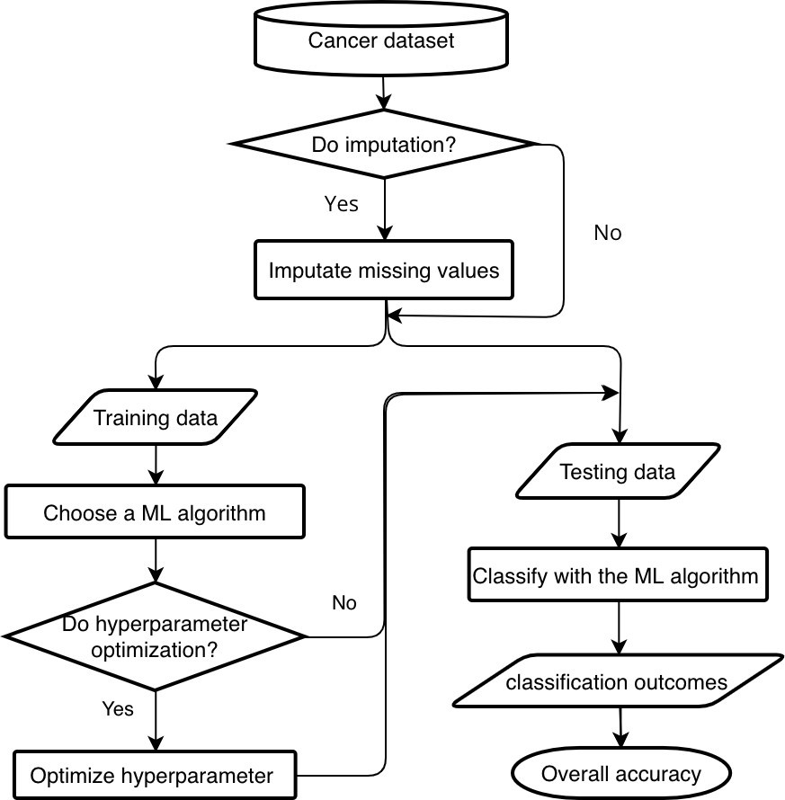
Figure 1 illustrates the workflow of prediction with application of imputation and hyperparameter optimization. False positives in detection refer to incorrectly classified negative instances as positives, while false negatives refer to incorrectly classified positive instances as negatives. In cancer diagnostics, the cost of false positives out weights the false negatives since the former put “patients at risk with invasive diagnostic procedures” [21].
In this study, we have chosen both Overall Accuracy and Area Under the Receiver Operating Characteristics (AUROC) [22] as metrics for evaluating the detection ac- curacy. The ROC curve is plotted with sensitivity against specificity: sensitivity is the ratio of true positives, defined as \(TPR = \frac{TP}{TP + FN’}\) and specificity is the proportion of true negatives, presented as \(FPR = \frac{FP}{TN + FP’}\) where TP stands for True Positive, TN True Negative, FP False Positive, and FN False Negative. A higher AUROC value indicates a better accuracy with a smaller false positive rate. An AUROC of 1.0 suggests a perfect classifier with 100% accuracy. The Overall Accuracy is calculated as the ratio of the number of correctly classified instances to the total number of instances, that is, \(\frac{TP + TN}{TP + TN + FP + FN’}.\)
The tests are implemented in Python 3.11 using the Scikit- learn [20] and Imbalanced Learn [23] libraries. They have been executed on a Dell Precision 5820 GPU workstation equipped with an Intel Xeon Processor (4 cores, 4.1 GHz) and an NVIDIA Quadro P2000 graphics card (5GB VRAM, 4 DisplayPort connectors).
3. Results
This section presents results from the four tests, including accuracy, execution time details in attached tables in the Appendix, along with AUROC curves. A summary of findings for each test is provided in Table 3.
The following three subsections provide details on how imputation, hyperparameter optimization, and the combination of these two methods impact machine learning algorithms’ prediction accuracy and execution time for cervical cancer diagnosis.
3.1. Impact of Imputation
We compare the two sets of results to determine the impact of imputation on the cervical cancer dataset. The first set includes the filtered dataset and imputed dataset without hyperparameter optimization for test 1 and test 3 (section 3.1.2). The second set includes the filtered dataset and imputed dataset with hyperparameter optimization for test 2 and test 4 (section 3.1.3).
3.1.1. Imputation Strategies
As mentioned in section 2.1, statistical and machine learning models are two popular imputation methods. In this study, both models have been explored for imputing the missing values in the cervical cancer dataset. Specifically, we have applied the statistical model using the most frequent value approach and the machine learning model using Random Forest for imputation, in both test 3 and test 4. Table 4 com- pares the Overall Accuracy and AUROC obtained through imputation using these two approaches in test 3 with 19 learning algorithms. The results indicate that imputation with Random Forest outperforms imputation with the most frequent value method, with 15 out of 19 algorithms demonstrating higher Overall Accuracy and 12 out of 19 algorithms showing better AUROC scores. In test 4 with 15 algorithms, the comparison between the two imputation approaches consistently indicates the better performance of the Random Forest approach. 13 out of 15 algorithms achieve better AUROC scores and 14 out of 15 algorithms obtain better Overall Accuracy. Thus, for the remainder of the paper, we report the findings based on imputation with Random Forest when imputation is applied.
3.1.2. Comparison of Results from Test 1 and Test 3
Table 5 and Table 7 report the results from test 1 and test 3, respectively. The comparisons of the accuracy and speed performance of the 19 machine learning algorithms on the filtered dataset and imputed dataset without hyperparameter optimization (Table 5 and Table 7) are described below.
- We have observed that all algorithms achieve higher Overall Accuracy with the imputed dataset compared to the filtered dataset, with improvements ranging from 0.40% to 3.42%. Six algorithms, including Ad a Boost, LightGBM, RF, RF-B, XGBoost, and LP, experience a decrease in AUROC scores ranging from 0.01 to 0.08 when using the imputed dataset compared to the filtered dataset. The remaining 13 algorithms show higher AUROC scores with the imputed dataset. Among them, LR, NB, NvSVM, and COPOD achieve a significant improvement of at least 0.14, with NuSVM achieving the highest improvement of 0.20. The other 9 algorithms show more modest improvements, limited to 0.09 or lower.
Table 2: List of Machine Learning Algorithms Examined
Type | Machine learning algorithms |
Unsupervised | Copula-Based Outlier Detection (COPOD) [24] K-Nearest Neighbor (KNN) [25] Subspace Outlier Detection (SUOD) [26] |
Semi-supervised | Self Training (ST) [27] Label Propagation (LP)[28] |
Supervised | Balanced Bagging [29] Adaptive Boosting (AdaBoost) [30] Balanced Random Forest [23] Light Gradient Boosting Machine (LightGBM) [31] Linear Discriminant Analysis (LDA) [32] Logistics Regression (LR) [33] Complement Naive Bayes (NB) [34] Neural Networks (NN) – Multi-Layer Perceptrons [35] ν-Support Vector Machines (NuSVM) [36] Random Forest (RF) [17] Support Vector Machine (SVM) [37] eXtreme Gradient Boosting (XGBoost) [38] |
- NN, RF-B, SVM and ST execute faster with the imputed dataset compared to the filtered dataset, resulting in saving more than 15% of execution time. BB, B-RF, and LR take slightly shorter execution time (ranging from 2% to 7%) with the imputed NB and CO- POD show similar execution times with both datasets. XGBoost, RF, SUOD and LR-B take slightly longer execution time (ranging from 3% to 9%) with the imputed dataset. The execution times of AdaBoost, LightGBM, LDA, NuSVM, LP, and KNN are much longer, ranging from 16% to 55%, on the imputed dataset compared to the filtered one.
3.1.3. Comparison of Results from Test 2 and Test 4
The findings from the comparisons of 15 algorithms’ accuracy and execution time on the filtered dataset and the imputed dataset with hyperparameter optimization (Table 6 and Table 8) indicate the following:
- All algorithms require longer execution time, ranging from 02 to 1.8 times, with the imputed dataset compared to the filtered one. Among them, SVM requires the longest additional time.
- All the tested algorithms demonstrate an improvement in Overall Accuracy with the imputed dataset, with the highest improvement being 3.27% (in LR). As for AUROC scores, RF and LightGBM experience a slight decrease of 0.03 and 0.04, respectively, when using the imputed dataset. The remaining algorithms show an improvement, with the highest improvement being 0.23 (in SVM).
3.2. Impact of hyperparameter optimization
To determine the impact of hyperparameter optimization on the cervical cancer dataset, we conduct a comparison between the two sets of results. The first set of results is from test 1 and test 2, and the second set is from test 3 and test 4. This study applies the grid search strategy to identify the optimal hyperparameter settings for an algorithm.
3.2.1. Comparison of Results from Test 1 and Test 2
Table 9 provides details of hyperparameter settings applied to the machine learning algorithms used in test 2, including 14 supervised learning and 1 semi-supervised learning. Table 5 and 6 report the results from test 1 and 2, respectively. Both tests have removed the missing values, while test 2 has also applied hyperparameter optimization. The following findings on prediction accuracy and speed are observed:
- The findings indicate that the application of hyper- parameter optimization does not significantly impact the Overall Accuracy of six algorithms: BB, AdaBoost, LightGBM, LDA, NN, and NuSVM. However, slight decreases in Overall Accuracy (ranging from 45% to 1.36%) are observed for B-RF, LR, RF and XGBoost, when hyperparameter optimization is applied. The remaining four algorithms demonstrate improved Over- all Accuracy with hyperparameter optimization. LR-B and LP show slight improvements (0.45% and 0.90%, respectively), while NB, RF-B, and SVM exhibit better improvements (ranging from 1.81% to 5.43%). Specifically, NB shows the highest improvement of 5.43%. Regarding AUROC scores, the performance of BB, B- RF, LDA, LR-B, NN, and NuSVMare the same with and without the application of hyperparameter optimization on this dataset. LP and LR experience a slight decrease in AUROC scores (ranging from 0.02 to 0.03) when hyperparameter optimization is applied compared to when it is not. The most significant de- crease decreases in the AUROC score are observed in NB and RF, with reductions of around 0.11.
Table 3: Summary of Results
Test No. | Description | Results |
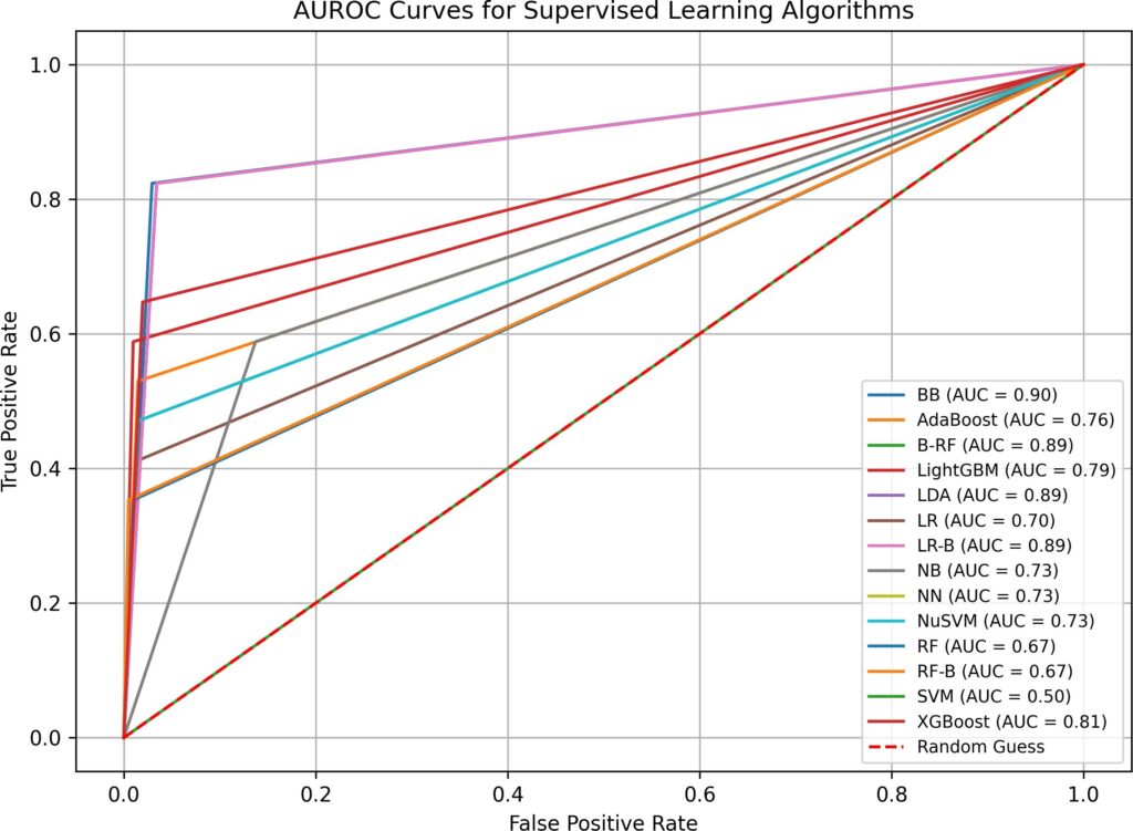
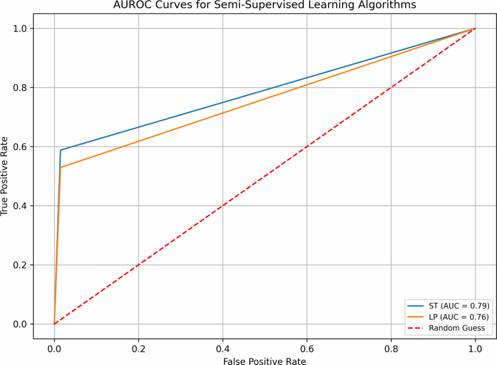
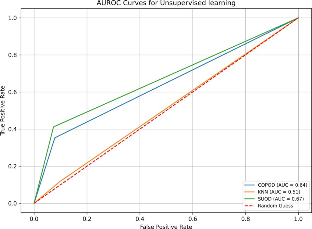
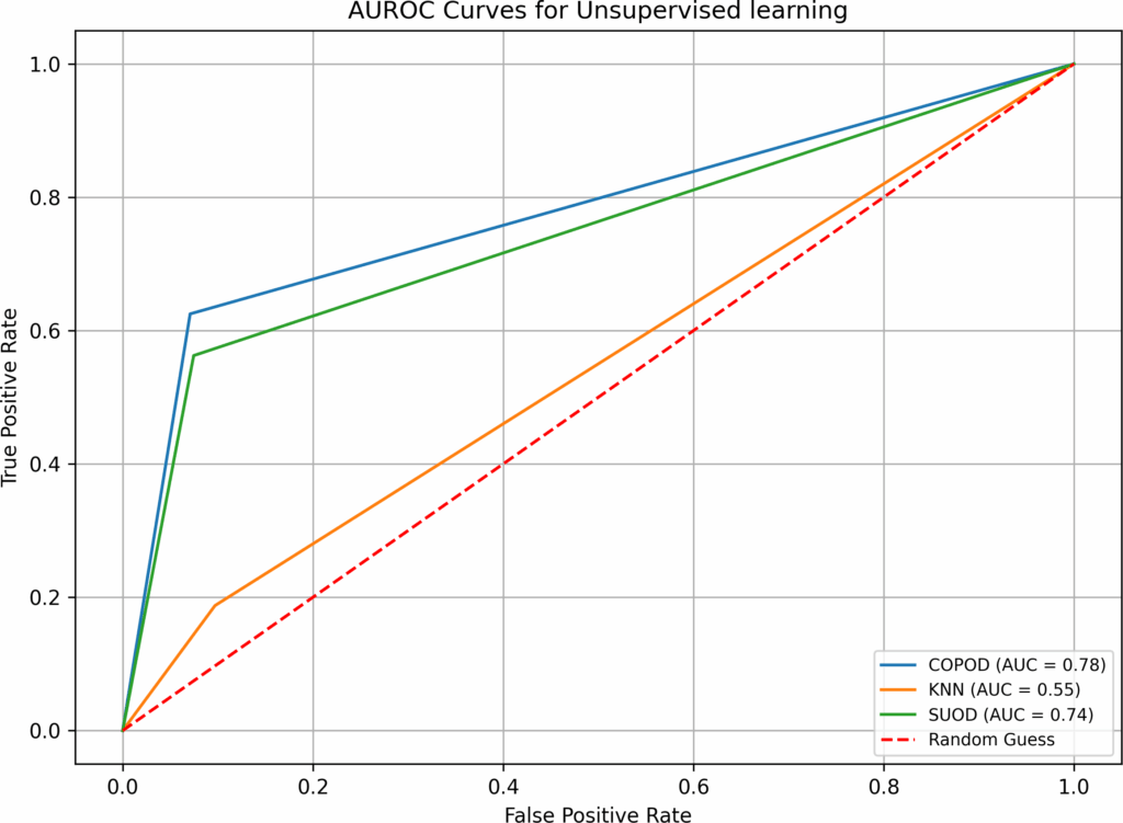
1 | 3 unsupervised; 2 semi-supervised; | Table 5 presents the details of the results from Test 1. |
14 supervised; | Overall, supervised learning algorithms have performed | |
No imputation; | the best in AUROC values, followed by semi-supervised, | |
No hyperparameter op. | and then unsupervised. 1 supervised learning (BB) has the highest AUROC score of 0.90, followed by 3 supervised | |
learning (B-RF, LDA and LR-B) with a score of 0.89; The | ||
highest Overall Accuracy of 95.93% is achieved by two su- | ||
pervised learning (BB and LightGBM), followed by one | ||
semi-supervised learning (ST) with accuracy of 95.48%. All | ||
19 algorithms have execution time of less than 0.77 second. | ||
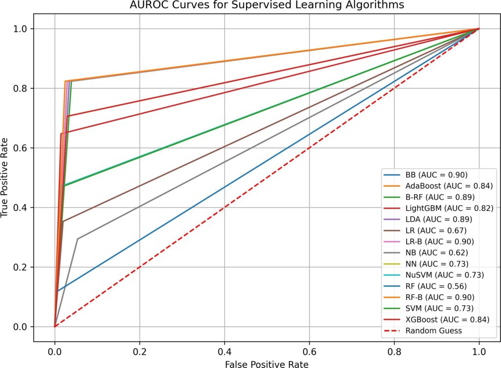
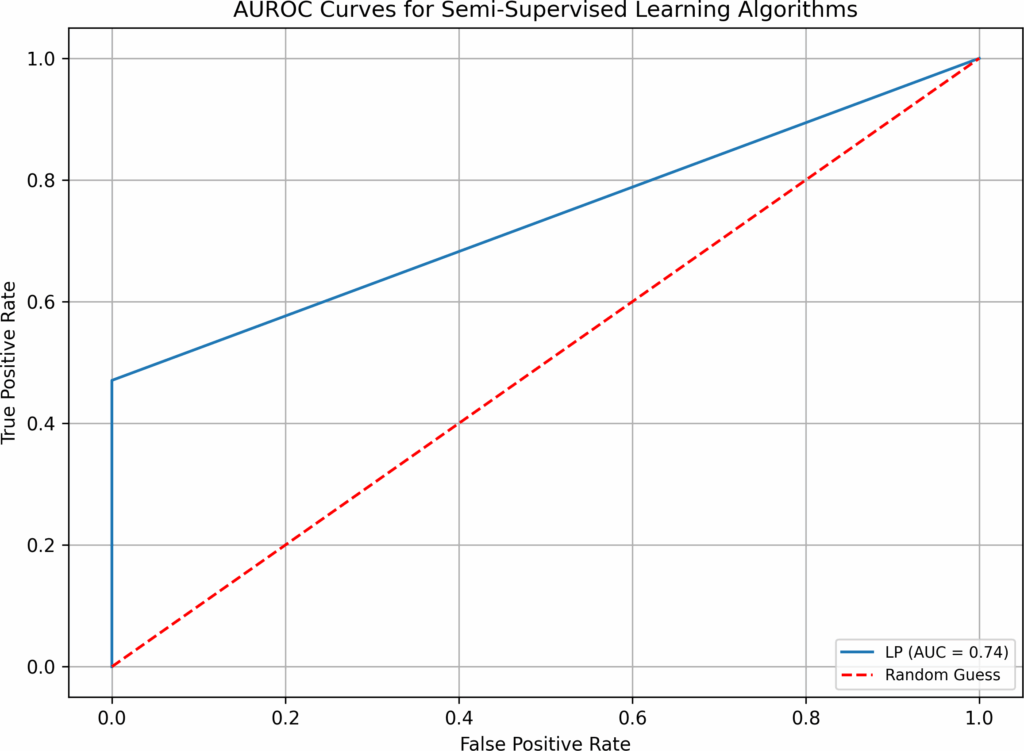
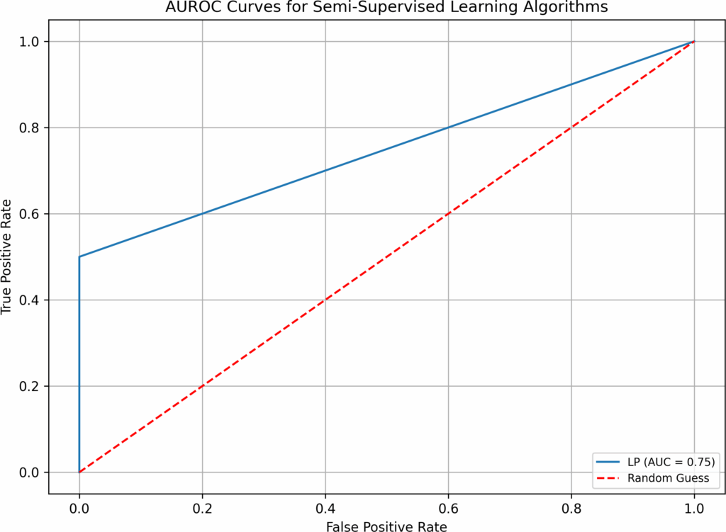
2 | 0 unsupervised; 1 semi-supervised; | Table 6 presents the details of the results from Test 2. |
14 supervised; | 5 supervised learning (BB, B-RF, LDA, LR-B and RF) have the | |
No imputation; | best AUROC values between 0.89 and 0.9, among which LDA | |
Hyperparameter op. | also has the one of the shortest processing time of only 0.37 second among all 15 algorithms. 13/14 supervised learning | |
have Overall Accuracy of over 92.76%. 3 supervised learning | ||
(BB, LightGBM, and LR-B) and 1 semi-supervised learning | ||
(LP) have the highest Overall Accuracy of 95.93%. LP also | ||
has one of the shortest execution times, taking 0.86 seconds. | ||
Only 4 algorithms have execution time of less than 1 second, | ||
5 algorithms take more than 30 seconds, and XGBoost has | ||
the longest execution time of 97.89 seconds. | ||
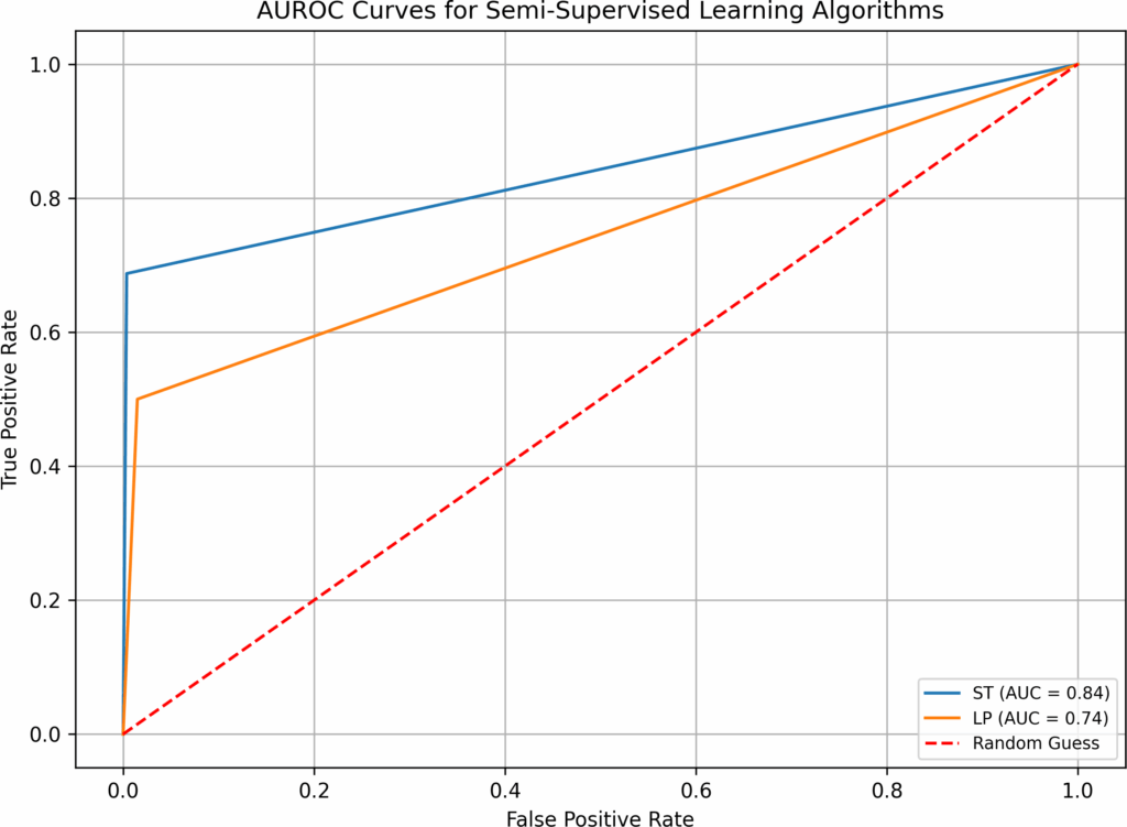
3 | 3 unsupervised; 2 semi-supervised; | Table 7 presents the details of the results from Test 3. |
14 supervised; | The top performers in AUROC are 4 supervised learning – | |
Imputation; | i.e., BB, B-RF, LDA, and LR-B with the values of 0.96, 0.95, | |
No hyperparameter op. | 0.95, and 0.95 respectively, among which LDA also has one of the shortest processing time(0.01 second). All but two | |
algorithms (KNN and NB) have Overall Accuracy higher | ||
than 90%. | ||
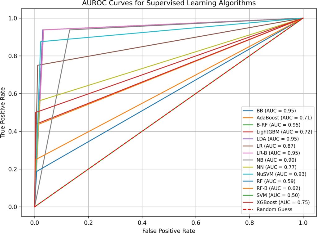
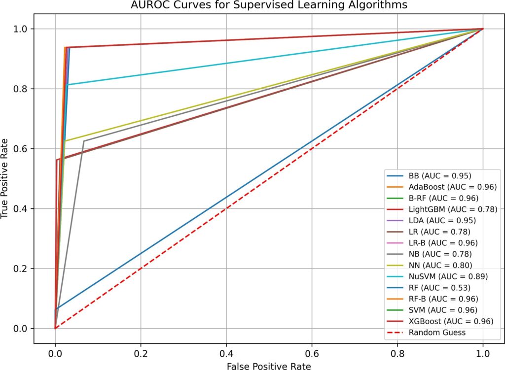
4 | 0 unsupervised; 1 semi-supervised; | Table 8 presents the details of the results from Test 4. |
14 supervised; | 8 out of 14 supervised learning (BB, AdaBoost, B-RF, LDA, | |
Imputation; | LR-B, RF-B, SVM, and XGBoost) have AUROC values be- | |
Hyperparameter op. | tween 0.95 and 0.96, among which LDA has the shortest execution time in test 4 (0.43 second). All 15 algorithms have | |
Overall Accuracy of over 91.5%, 11 of them have processing | ||
time more than 1 second among which XGBoost has the | ||
longest execution time of 105.23 second. |
- With the application of hyperparameter optimization, all tested algorithms experience considerably longer execution times compared to their counterparts without optimization. NB, LDA, LR-B, NN, and NuSVM take over less than 50 times longer to execute, with NB taking 9 times longer as the shortest. LR takes more than 50 times but less than 68 times longer to The remaining algorithms take much longer to exe- cute, ranging from 161 (LP) to 1240 times (XGBoost), when hyperparameter optimization is applied.
3.2.2. Comparison of Results from Test 3 and Test 4
Table 7 and Table 8 present the results of test 3 and test 4, respectively. In both tests, imputation has been applied to the dataset, with hyperparameter optimization being applied in test 4, but not in test 3. Table 10 describes the hyperparameter settings applied to the machine learning algorithms used in test 4, including 14 supervised learning and 1 semi-supervised learning.
- The application of hyperparameter optimization does not impact the Overall Accuracy for LDA, NN, and
RF; the result remains the same regardless of whether it is applied. BB, LR, and NuSVM experience slight decrease in Overall Accuracy, ranging from 0.35% (BB) to 1.06% (LR). The remaining algorithms show improvements in Overall Accuracy at different levels. B-RF, Light GBM, and XGBoost have slight increase (<=0.7%). AdaBoost and LP have an increase over 1% but less than 2%. RF-B, SVM, and NB show better im- provement, increasing in the range of 2.11% to 4.23%, with NB receiving the highest improvement.
The AUROC scores of BB, B-RF, LDA, and LR-B are not affected by whether the optimization is applied to the dataset. However, other algorithms show an impact from the optimization. LR, NB, NuSVM, and RF experience a reduction in scores, ranging from 0.03 to 0.12, when optimization is applied. The other seven algorithms demonstrate an improvement in AUROC scores with the optimization. LP, NN, and LightGBM show a slight improvement of 0.01, 0.03, and 0.06, re- spectively, while AdaBoost, XGBoost, RF-B, and SVM show an increase ranging from 0.21 to 0.46, with SVM achieving the highest improvement of 0.46.
Table 4: Imputation with Most Frequent Value vs. Random Forest
Algorithms | Imputation (Most Frequent) | Imputation | (Random Forest) | |
Overall(%) | AUROC | Overall(%) | AUROC | |
BB | 95.07 | 0.92 | 97.18 | 0.96 |
AdaBoost | 93.66 | 0.68 | 95.77 | 0.74 |
B-RF | 95.77 | 0.93 | 96.13 | 0.95 |
LightGBM | 95.77 | 0.74 | 96.83 | 0.72 |
LDA | 96.48 | 0.93 | 96.83 | 0.95 |
LR | 96.13 | 0.75 | 97.54 | 0.87 |
LR-B | 95.42 | 0.87 | 96.48 | 0.95 |
NB | 89.44 | 0.74 | 87.32 | 0.90 |
NN | 94.72 | 0.66 | 95.42 | 0.74 |
NuSVM | 95.77 | 0.74 | 96.83 | 0.92 |
RF | 96.48 | 0.77 | 96.48 | 0.75 |
RF-B | 95.42 | 0.66 | 94.72 | 0.56 |
SVM | 93.66 | 0.50 | 94.37 | 0.50 |
XGBoost | 95.42 | 0.77 | 96.83 | 0.75 |
ST | 96.82 | 0.79 | 98.94 | 0.91 |
LP | 96.11 | 0.73 | 95.76 | 0.74 |
COPOD | 90.81 | 0.76 | 89.25 | 0.71 |
KNN | 87.99 | 0.63 | 87.10 | 0.65 |
SUOD | 90.11 | 0.73 | 89.25 | 0.71 |
- Similar to the observation described in section 2.1 about the significant increase in speed when hyperparameter optimization is applied, all algorithms in test 4 take significantly longer to execute, ranging from 23 to 1450 times longer, with LDA requiring the shortest additional time (23) and SVM requiring the longest (1450) compared to without hyperparameter optimization.
3.3. Impact of hyperparameter optimization and imputation
The impact of applying both hyperparameter optimization and imputation is evaluated based on the findings from test 1 (Table 5) and test 4 (Table 8) in appendix section.
The results indicate that the application of both hyperparameter optimization and imputation has a positive impact on the detection accuracy, including both Overall Accuracy and AUROC scores.
Overall Accuracy improves for all algorithms when both techniques are applied. BB and RF show a slight improvement of around 0.6%. B-RF, LightGBM, LDA, LR-B, NN, NuSVM, and XGBoost demonstrate increases ranging from 1% to 1.91%. AdaBoost, LR, NB, LP, RF-B, and SVM show higher accuracy improvements of over 2%), with SVM and NB achieving significant increases of 4.88% and 7.39%, re- spectively.
AUROC scores are improved for most algorithms except for LightGBM, LP, and RF, which experience a slight de- crease ranging from 0.01 to 0.14. BB, B-RF, LDA, LR-B, NB, and NN demonstrate a slight increase, with values ranging from 0.05 to 0.08. The remaining algorithms, including AdaBoost, RF-B, SVM, and XGBoost, receive increases ranging from 0.14 to a maximum of 0.46 (SVM).
The application of both approaches significantly in- creases the execution time for all algorithms. Consistent with the findings in sections 3.2.1 and 3.2.2, the execution time of each algorithm increases ranging from 10 to 1342 times compared to when neither approach is applied. NB takes the shortest additional time (10 times), while XGBoost takes the longest time (1342 times) compared to when the approaches are not used.
3.3. Discussion
In this study, we are interested in comparing the performance of machine learning applications in cancer diagnosis, especially approaches that are flexible enough to detect different kinds of cancers without compromising accuracy. To achieve this goal, we have examined the impact of imputation and hyperparameter optimization on the performance of algorithms using a cervical cancer dataset. Three criteria execution speed, overall diagnosis accuracy, and AUROC scores are used to evaluate performance. Since the cost of false positive is high in cancer diagnosis, and a good AUROC score indicates low false positive rate, it is a more important criteria in this study. Based on whether imputation and hyperparameter optimization is included, we have split the algorithms into four tests.
Missing values are common in medical data, and statistical and machine learning are two popular methods that handle missing data. By comparing the performance of Random Forest, a common machine learning method, and the most frequent value method in statistics, we found that machine learning approach outperforms statistical approach as an imputation method in this study. This finding echoes with our discussion in section 2.1 that machine learning is well suited to process dataset with missing values, especially when the dataset is small.
Results of this study show that the four top performers are all supervised learning: BB, B-RF, LDA, and LR-B, among which the performance of LDA is especially noticeable by consistently delivering the most accurate diagnosis within the shortest time across all four tests. These four supervised learning definitely merit more attention in future studies.
Examination of findings from the four tests shows the following:
- when both imputation and hyperparameter optimization are absent in test 1, supervised and semi-supervised learning have performed well in Overall Accuracy, 15 out of 16 algorithms have scored over 31%. However, in terms of AUROC, the top performers (BB, B-RF, LDA, and LR-B) only have AUROC value of 0.89, none has values over 0.9. SVM, a popular supervised learning algorithm, has performed the worst: its AUROC value is only 0.5. Unsupervised learning algorithms have not performed well, all three have AUROC values below 0.7. Although the execution time in test 1 is fast(none is over 0.77 second), the overall low AUROC values is definitely not satisfactory.
- To examine the impact of imputation, we have con- ducted two One set of comparison is between results from test 1 and test 3 The result shows that when only imputation is applied, the change in execution time is marginal and yet the improvement of Overall Accuracy and AUROC is impressive compared to when both methods are absent. All algorithms have increased the Overall Accuracy, and 68% of the algorithms have improved on their AUROC scores. The other set of comparison is between results from test 2 and test 4. When both imputation and hyperparameter optimization are applied, compared to when only hyper- parameter optimization is applied, all 15 algorithms have increased their execution times. The good news is that the Overall Accuracy of all algorithms has improved, and most AUROC values have increased. These two sets of comparisons suggest that the employment of imputation could improve the prediction accuracy without extending the execution time.
- To evaluate the impact of hyperparameter optimization, we have also carried out two set of One set of comparison is between test 1 and 2. When only hyperparameter optimization is applied in test 2, the execution time of all algorithms have increased significantly than when both methods are absent (test 1). 11 out of 15 algorithms have execution time of more than 1 second whereas none of the algorithms has run time over 1 second when both methods are absent in test 1. XGBoost in test 2 even has run time as high as 97 seconds. 7 algorithms have increased their Overall Accuracy and 8 out of 15 algorithms have improved their AUROC scores. The other set of comparison is between test 3 and 4. The results show that when both methods are present (test 4), the execution time for majority of the algo- rithms is significantly longer than when only imputation is present (test 3): only 4 algorithms have execution time of less than 1 second in test 4, whereas all but 2 algorithms have less than 1 second in test 3. 9 algorithms have improved their Overall Accuracy and AUROC scores, among which the AUROC score improvements are especially noticeable for three supervised learning algorithms: RF-B, SVM, XG- Boost, with improvement of 28%, 92%, and 71% respectively. The findings from these two sets of comparisons show that inclusion of hyperparameter optimization could lengthen the execution time while improving the prediction accuracy, especially for some algorithms such as RF-B, SVM, and XGBoost.
- Comparison of all 4 tests shows that overall, the inclusion of both imputation and hyperparameter optimization does deliver the best AUROC values, with 53% score more than 95 and 0.96, whereas none from test 1, 20% from test 2, 21% from test 3 has such values. To summarize, our study has shown how the application of both imputation and hyperparameter optimization methods in machine learning could improve the detection accuracy. Also, by taking all features of the data into consideration, although the diagnosis accuracy of the classifier is not as high as 99%-100% as observed in other systems that apply various feature selection [12], the performance is satisfactory with the inclusion of both imputations and hyperparameters optimization. In addition, by not having feature selection, the classifier can avoid the overfitting problems that are common in many studies, and can potentially be applied in diagnosing various types of cancers. This study does come with its limitations. Firstly, al- though we have examined as many as 19 different machine learning algorithms, most are supervised learning algorithms with only two being semi-supervised and three being unsupervised. To gain comprehensive understanding on the performance differences among different types of algorithms, it would be better to consider more semi- supervised and unsupervised machine algorithms in future studies. Secondly, one cervical cancer dataset is applied to evaluate the diagnosis performance of different algorithms. To improve the generalizability of the findings, we will use cervical cancer datasets from different sources upon the data availability. Also, to investigate whether how algorithms dif- fer from each other, it would be advisable to include datasets with various types of cancers for evaluation. Thirdly, the dataset used in this study is text based. Since images are extensively used in cancer diagnosis, it would be preferable to include image-based datasets in further studies.
4. Conclusion
With the increasing popularity of machine learning applications in cancer diagnosis, there has been a need to evaluate the performance of these algorithms and identify approaches that could improve their performance. This study contributes to the literature by examining the cancer detection performance of as many as 19 supervised, semi-supervised, unsupervised learning machine learning algorithms. To investigate ways that expand the types of cancers that the algorithms could accurately detect, this study has investigated how the inclusion and exclusion of imputation and hyperparameter optimization would impact performance using a cervical cancer dataset. The results suggest that applying both hyperparameter optimization and imputation methods could impact detection performance much better than employing each of them independently or none of them. This study has provided insights on creating versatile classifiers that could deliver solid results.
5. Availability of data and materials
The cervical cancer dataset that the current study has analyzed are openly available in UCI Machine Learning Repository, the web address is https://archive.ics.uci.edu/ ml/datasets/Cervical+cancer+%28Risk+Factors%29.
Conflict of Interest The authors declare no conflict of interest.
Annexure
Table 5: Results – Test 1
Algorithm | Time (sec) | False Neg. | False Pos. | Correct /221 | Overall (%) | AUROC |
BB | 0.03 | 3 | 6 | 212 | 95.93% | 0.90 |
AdaBoost | 0.06 | 8 | 3 | 210 | 95.02% | 0.76 |
B-RF | 0.22 | 3 | 7 | 211 | 95.48% | 0.89 |
LightGBM | 0.06 | 7 | 2 | 212 | 95.93% | 0.79 |
LDA | 0.02 | 3 | 7 | 211 | 95.48% | 0.89 |
LR | 0.06 | 10 | 3 | 208 | 94.12% | 0.70 |
LR-B | 0.10 | 3 | 7 | 211 | 95.48% | 0.89 |
NB | 0.02 | 7 | 28 | 186 | 84.16% | 0.73 |
NN | 0.93 | 9 | 3 | 209 | 94.57% | 0.73 |
NuSVM | 0.02 | 9 | 3 | 209 | 94.57% | 0.73 |
RF | 0.14 | 11 | 2 | 208 | 94.12% | 0.67 |
RF-B | 0.16 | 11 | 1 | 209 | 94.57% | 0.67 |
SVM | 0.02 | 17 | 0 | 204 | 92.31% | 0.50 |
XGBoost | 0.08 | 6 | 4 | 211 | 95.48% | 0.81 |
LP | 0.01 | 8 | 3 | 210 | 95.02% | 0.76 |
ST | 0.01 | 7 | 3 | 211 | 95.48% | 0.79 |
COPOD | 0.01 | 16 | 11 | 194 | 87.78% | 0.64 |
KNN | 0.01 | 20 | 15 | 186 | 84.16% | 0.51 |
SUOD | 1.03 | 15 | 10 | 196 | 88.69% | 0.67 |
Note: imputation (no), hyperparameter optimization (no).
Table 6: Results – Test 2
Algorithm | Time (sec) | False Neg. | False Pos. | Correct /221 | Overall (%) | AUROC |
BB | 6.94 | 3 | 6 | 212 | 95.93% | 0.90 |
AdaBoost | 22.09 | 5 | 6 | 210 | 95.02% | 0.84 |
B-RF | 59.91 | 3 | 8 | 210 | 95.02% | 0.89 |
LightGBM | 21.50 | 6 | 3 | 212 | 95.93% | 0.82 |
LDA | 0.37 | 3 | 7 | 211 | 95.48% | 0.89 |
LR | 4.40 | 11 | 4 | 206 | 93.21% | 0.67 |
LR-B | 4.09 | 3 | 6 | 212 | 95.93% | 0.90 |
NB | 0.21 | 12 | 11 | 198 | 89.59% | 0.62 |
NN | 46.09 | 9 | 3 | 209 | 94.57% | 0.73 |
NuSVM | 0.79 | 9 | 3 | 209 | 94.57% | 0.73 |
RF | 34.65 | 15 | 1 | 205 | 92.76% | 0.56 |
RF-B | 34.14 | 3 | 5 | 213 | 96.38% | 0.90 |
SVM | 5.22 | 9 | 4 | 208 | 94.12% | 0.73 |
XGBoost | 96.89 | 5 | 6 | 210 | 95.02% | 0.84 |
LP | 0.86 | 9 | 0 | 212 | 95.93% | 0.74 |
Note: imputation(no), hyperparameter optimization(yes).
Table 7: Results – Test 3
Algorithm | Time (sec) | False Neg. | False Pos. | Correct /284 | Overall (%) | AUROC |
BB | 0.03 | 1 | 8 | 275 | 96.83% | 0.95 |
AdaBoost | 0.08 | 9 | 4 | 271 | 95.42% | 0.71 |
B-RF | 0.20 | 1 | 9 | 274 | 96.48% | 0.95 |
LightGBM | 0.08 | 9 | 1 | 274 | 96.48% | 0.72 |
LDA | 0.02 | 1 | 8 | 275 | 96.83% | 0.95 |
LR | 0.06 | 4 | 3 | 277 | 97.54% | 0.87 |
LR-B | 0.11 | 1 | 9 | 274 | 96.48% | 0.95 |
NB | 0.02 | 1 | 35 | 248 | 87.32% | 0.90 |
NN | 0.80 | 7 | 5 | 272 | 95.77% | 0.77 |
NuSVM | 0.02 | 2 | 6 | 276 | 97.18% | 0.93 |
RF | 0.15 | 13 | 2 | 269 | 94.72% | 0.59 |
RF-B | 0.11 | 12 | 1 | 271 | 95.42% | 0.62 |
SVM | 0.01 | 16 | 0 | 268 | 94.37% | 0.50 |
XGBoost | 0.08 | 8 | 1 | 275 | 96.83% | 0.75 |
LP | 0.01 | 8 | 4 | 272 | 95.77% | 0.74 |
ST | 0.01 | 5 | 1 | 278 | 97.89% | 0.84 |
COPOD | 0.01 | 19 | 6 | 259 | 91.20% | 0.78 |
KNN | 0.02 | 26 | 13 | 245 | 86.27% | 0.55 |
SUOD | 1.12 | 20 | 7 | 257 | 90.49% | 0.74 |
Note: imputation(yes), hyperparameter optimization (no).
Table 8: Results – Test 4
Algorithm | Time (sec) | False Neg. | False Pos. | Correct /284 | Overall (%) | AUROC |
BB | 7.08 | 1 | 9 | 274 | 96.48% | 0.95 |
AdaBoost | 26.88 | 1 | 7 | 276 | 97.18% | 0.96 |
B-RF | 63.50 | 1 | 7 | 276 | 97.18% | 0.96 |
LightGBM | 26.69 | 7 | 1 | 276 | 97.18% | 0.78 |
LDA | 0.43 | 1 | 8 | 275 | 96.83% | 0.95 |
LR | 4.80 | 7 | 3 | 274 | 96.48% | 0.78 |
LR-B | 5.24 | 1 | 7 | 276 | 97.18% | 0.96 |
NB | 0.22 | 6 | 18 | 260 | 91.55% | 0.78 |
NN | 68.49 | 6 | 6 | 272 | 95.77% | 0.80 |
NuSVM | 0.86 | 3 | 7 | 274 | 96.48% | 0.89 |
RF | 36.07 | 15 | 0 | 269 | 94.72% | 0.53 |
RF-B | 37.11 | 1 | 6 | 277 | 97.54% | 0.96 |
SVM | 14.64 | 1 | 7 | 276 | 97.18% | 0.96 |
XGBoost | 104.79 | 1 | 7 | 276 | 97.18% | 0.96 |
LP | 0.93 | 8 | 0 | 276 | 97.18% | 0.75 |
Note: imputation (yes), hyperparameter optimization (yes).
Table 9: Hyperparameter Setting for test 2
Algorithm | Hyperparameter setting |
BB AdaBoost B-RF LightGBM LDA LR LR-B NB NN NuSVM RF RF-B SVM XGBoost LP | ’n_estimators’: 100 ’learning_rate’: 0.01, ’n_estimators’: 300 ’criterion’: ’gini’, ’max_depth’: 1, ’n_estimators’: 500 ’learning_rate’: 0.1, ’max_depth’: 10, ’n_estimators’: 100, ’scale_pos_weight’: 6 ’solver’: ’svd’, ’tol’: 0.0001 ’C’: 100, ’penalty’: ’l2’, ’solver’: ’newton-cg’ ’C’: 1.0, ’penalty’: ’l2’, ’solver’: ’liblinear’ ’alpha’: 9 ’activation’: ’relu’, ’alpha’: 0.05, ’hidden_layer_sizes’: (10, 30, 10), ’learning_rate’: ’adaptive’, ’solver’: ’adam’ ’gamma’: 0.001, ’nu’: 0.1 ’criterion’: ’gini’, ’max_depth’: 5, ’n_estimators’: 500 ’criterion’: ’entropy’, ’max_depth’: 3, ’n_estimators’: 200 ’C’: 1.0, ’gamma’: 0.001, ’kernel’: ’linear’ ’colsample_bytree’: 1.0, ’gamma’: 2, ’max_depth’: 3, ’min_child_weight’: 1, ’subsample’: 1.0 ’gamma’: 0.1, ’kernel’: ’knn’, ’n_neighbors’: 3 |
Table 10: Hyperparameter settings for test 4
Algorithm | Hyperparameter setting |
BB AdaBoost B-RF LightGBM LDA LR LR-B NB NN NuSVM RF RF-B SVM XGBoost LP | ’n_estimators’: 100 ’learning_rate’: 0.001, ’n_estimators’: 100 ’criterion’: ’gini’, ’max_depth’: 1, ’n_estimators’: 200 ’learning_rate’: 0.1, ’max_depth’: 10, ’n_estimators’: 100, ’scale_pos_weight’: 6 ’solver’: ’svd’, ’tol’: 0.1 ’C’: 1.0, ’penalty’: ’l2’, ’solver’: ’liblinear’ ’C’: 0.1, ’penalty’: ’l2’, ’solver’: ’newton-cg’ ’alpha’: 9 ’activation’: ’relu’, ’alpha’: 0.0001, ’hidden_layer_sizes’: (20,), ’learning_rate’: ’constant’, ’solver’: ’adam’ ’gamma’: 0.01, ’nu’: 0.1 ’criterion’: ’entropy’, ’max_depth’: 3, ’n_estimators’: 200 ’criterion’: ’gini’, ’max_depth’: 3, ’n_estimators’: 500 ’C’: 1.0, ’gamma’: 0.001, ’kernel’: ’linear’ ’colsample_bytree’: 0.8, ’gamma’: 1.5, ’max_depth’: 3, ’min_child_weight’: 10, ’subsample’: 1.0 ’gamma’: 0.1, ’kernel’: ’knn’, ’n_neighbors’: 3 |
- World Health Organization, “Cancer: Key facts,” https://www.who.int/news-room/fact-sheets/detail/cancer, 2022.
- World Health Organization, “Global Strategy on Human Resources for Health: Workforce 2030: Reporting at Seventy-fifth World Health Assembly,” https://www.who.int/news/item/ 02-06-2022- global-strategy-on-human-resources-for-health–workforce-2030, 2022.
- J. A. Cruz and D. S. Wishart, “Applications of Machine Learning in Cancer Prediction and Prognosis”. Cancer Informatics 2, p:59–77, 2006. DOI: 10.1177/117693510600200030
- K. Wan, C. H. Wong, H. F. Ip, D. Fan, P. L. Yuen, H. Y. Fong, and
M. Ying, “Evaluation of the Performance of Traditional Machine Learning Algorithms, Convolutional Neural Network and Automl Vision in Ultrasound Breast Lesions Classification: a Comparative Study,” Quantitative imaging in medicine and surgery, vol. 11, no. 4, pp:1381–1393, 2021. DOI: 10.21037/qims-20-922 - S. Hussein, P. Kandel, C. W. Bolan, M. B. Wallace, and U. Bagci, “Lung and Pancreatic Tumor Characterization in the Deep Learning Era: Novel Supervised and Snsupervised Learning Approaches,” IEEE Transactions on Medical Imaging, vol. 38, pp:1777–1787, 2019.
- K. Fernandes, J. S. Cardoso, and J. C. Fernandes, “Transfer learn- ing with partial observability applied to cervical cancer screening,” in Iberian Conference on Pattern Recognition and Image Analysis, 2017. DOI: 10.1007/978-3-319-58838-4_27
- Intel-mobileodt, “Intel & MobileODT Cervical Cancer Screen-s://kaggle.com/competitions/intel-mobileodt-cervical-
cancer-screening, 2017. - M. M. Ali, K. Ahmed, F. M. Bui, B. K. Paul, S. M. Ibrahim, J.
M. W. Quinn, and M. A. Moni, “Machine Learning-based Sta- tistical Analysis for Early Stage Detection of Cervical Cancer,” Computers in Biology and Medicine, vol. 139, no. 104985, 2021.
DOI: 10.1016/j.compbiomed.2021.104985 - W. William, J. A. Ware, A. H. Basaza-Ejiri, and J. Obungoloch, “A Review of Image Analysis and Machine Learning Techniques for Automated Cervical Cancer Screening from Pap-smear Im- ages,” Computer Methods and Programs in Biomedicine, vol. 164, pp:15-22, 2018. DOI: 10.1016/j.cmpb.2018.05.034
- J. Lu, E. Song, A. Ghoneim, and M. Alrashoud, “Machine Learn- ing for Assisting Cervical Cancer Diagnosis: An Ensemble Ap- proach,” Future Generation Computer Systems, vol. 106, pp:199- 205, 2020. DOI: 10.1016/j.future.2019.12.033
- C. Luo, B. Liu, and J. Xia, “Comparison of Several Machine Learning Algorithms in the Diagnosis of Cervical Cancer,” in Inter- national Conference on Frontiers of Electronics, Information and Computation Technologies, 2021. DOI: 10.1145/3474198.3478165
- B. Nithya and V. Ilango, “Evaluation of Machine Learning Based Optimized Feature Selection Approaches and Classification Meth- ods for Cervical Cancer Prediction,” SN Applied Sciences vol. 1, 1–16, 2019. DOI: 10.1007/s42452-019-0645-7
- Y. R. Park, Y. J. Kim, W. Ju, K. Nam, S. Kim, and K. G. Kim, “Comparison of Machine and Deep Learning for the Classification of Cervical Cancer Based on Cervicography Images,” Scientific Reports, vol. 11, 2021. DOI: 10.1038/s41598-021-95748-3
- D. B. Rubin, “Multiple Imputation After 18+ Years,” Journal of the American Statistical Association, vol. 91, pp. 473–489, 1996.
DOI: 10.1080/01621459.1996.10476908 - M. Feurer, F. Hutter, “Hyperparameter optimization,” in: F. Hutter, L. Kotthoff, J. Vanschoren (Eds.), Automatic Machine Learning: Methods, Systems, Challenges, Springer, pp. 3–38, 2019.
DOI: 10.1007/978-3-030-05318-5_1 - J. Bergstra, R. Bardenet, Y. Bengio, and B. K´egl, “Algorithms for hyper-parameter optimization,” Advances in Neural Information Processing systems, vol. 24, 2011.
- L. Breiman, “Random Forests,” Machine Learning, vol. 45 pp. 5–32, 2004. DOI: 10.1023/A:1010933404324
- L. Breiman, J. H. Friedman, R. A. Olshen, C. J. Stone, “Classifi- cation and Regression Trees,” Brooks/Cole Publishing, Monterey, 1984. DOI: 10.1201/9781315139470
- Mayo, “Biopsy: Types of Biopsy Procedures Used to Diagnose Cancer,” https://www.mayoclinic.org/diseases-conditions/cancer/ in-depth/biopsy/art-20043922, 2021.
- O. Kramer, “Scikit-learn,” In: Machine Learning for Evolution Strategies, pp. 45–53. Springer, 2016. DOI: 10.1007/978-3-319- 33383-0_5
- J. Huo, Y. Xu, T. Sheu, R. Volk, and Y. Shih, “Complication Rates and Downstream Medical Costs Associated with Invasive Diagnostic Procedures for Lung Abnormalities in the Community Setting,” JAMA Internal Medicine vol. 179, no. 3, pp. 324-332, 2019. DOI: 10.1001/jamainternmed.2018.6277
- J. A. Hanley, B. J. McNeil, “The Meaning and Use of the Area Under a Receiver Operating Characteristic (ROC) Curve,” Ra- diology, vol. 143, no. 1, pp. 29–36, 1982. DOI: 10.1148/radiol- ogy.143.1.7063747
- ImbalancedLearn, “Balanced Random Forest Classifier,” https://imbalanced- learn.org/stable/references/generated/imblearn. ensemble.BalancedRandomForestClassifier.html, 2022.
- Z. Li, Y. Zhao, N. Botta, C. Ionescu, and X. Hu, “COPOD: Copula-Based Outlier Detection,” in Proceedings of IEEE Interna-
Mining (ICDM), pp. 1118–1123, 2020.
DM50108.2020.00135 - N. S. Altman, “An Introduction to Kernel and Nearest-Neighbor Nonparametric Regression,” The American Statistician, vol. 46, no.3, pp.175-185, 1992. DOI: 10.1080/00031305.1992.10475879
- Y. Zhao, X. Hu, C. Cheng, C. Wang, C. Wan, W. Wang, J. Yang, H. Bai, Z. Li, C. Xiao, and Y. Wang, “SUOD: Accelerating Large-Scale Unsupervised Heterogeneous Outlier Detection,” in Proceedings of Machine Learning and Systems, vol. 3, pp.463-478, 2021.
- D. Yarowsky, “Unsupervised Word Sense Disambiguation Rival- ing Supervised Methods,” In 33rd Annual Meeting of the Asso- ciation for Computational Linguistics, pp. 189-196, 1995. DOI: 10.3115/981658.981684
- X. ZhuГ´ and Z. GhahramaniГ´н, “Learning from Labeled and Unlabeled Data with Label Propagation,” ProQuest Number: IN- FORMATION TO ALL USERS, 2002.
- A. Lazarevic, V. Kumar, “Feature Bagging for Outlier Detection,” In: Proceedings of the Eleventh ACM SIGKDD International Conference on Knowledge Discovery in Data Mining, 2005. DOI: 10.1145/1081870.1081891
- Y. Freund, R. E. Schapire, “A Decision-Theoretic Generalization of On-line Learning and an Application to Boosting,” In: Vit´anyi, P. (ed.) Computational Learning Theory, pp. 23–37. Springer, Berlin,
Heidelberg, 1995. DOI: 10.1006/jcss.1997.1504 - G. Ke, M. Qi Meng, T. Finley, T. Wang, W. Chen, W. Ma, Q. Ye, and T. Liu, “Lightgbm: A highly Efficient Gradient Boosting De- cision Tree,” Advances in Neural Information Processing Systems, vol. 30, 2017.
- A. J. Izenman, “Linear Discriminant Analysis,” Springer New York, New York, NY, pp. 237–280, 2008. DOI: 10.1007/978-0-387- 78189-1_8
- W. Chen, Y. Chen, Y. Mao, B.-L. Guo, “Density-based Logistic Regression,” in Proceedings of the 19th ACM SIGKDD interna- tional conference on Knowledge Discovery and Data Mining, pp. 140-148, 2013. DOI: 10.1145/2487575.2487583
- J. D. Rennie, L. Shih, J. Teevan, D. R. Karger, “Tackling the Poor Assumptions of Naive Bayes Text Classifiers,” in Proceedings of the 20th International Conference on Machine Learning (ICML-03), pp. 616–623, 2003.
- M. Popescu, V. E. Balas, L. Perescu-Popescu, and N. E. Mas- torakis, “Multilayer Perceptron and Neural Networks,” WSEAS Transactions on Circuits and Systems, vol. 8, no. 7, pp. 579-588, 2009.
- P.-H. Chen, C.-J. Lin, and B. Scho¨lkopf, “A tutorial on ν-Support Vector Machines,” Applied Stochastic Models in Business and Industry, vol. 21, no. 2, pp. 111–136, 2005. DOI: 10.1002/asmb.537
- C. Cortes and V. N. Vapnik, “Support-Vector Networks,” Machine Learning, vol. 20, 273–297, 1995. DOI: 10.1007/BF00994018
- T. Chen and C. Guestrin, “Xgboost: A Scalable Tree Boosting System,” in Proceedings of the 22nd ACM SIGKDD International owledge Discovery and Data Mining, 2016. DOI:
39672.2939785