Information extracted from remote sensing data can be applied to monitor the business and natural environments of a geographic area. Although a wide range of classical machine learning techniques have been utilized to obtain such information, their performance differs greatly in classification accuracy. In this study, we aim to examine whether quantum-enhanced machine learning can improve the performance of classical machine learning algorithms in binary classifications of satellite remote sensing data. Using 16 pre-labeled datasets, we apply Support Vector Machine-quantum annealing solver (SVM-QA) – a type of quantum machine learning algorithm, with optimized (Gamma) value on the task of image classification and compare its results with the top performers of classical machine learning algorithms. The results show that in 10 out of 16 datasets, the hyper parameterized SVM-QA classifier outperforms the best classical machine learning algorithms in terms of classification accuracy. The findings suggest the potentiality of quantum computing in remote sensing. This study contributes to the literature of remote sensing image data classification and applications of quantum machine learning for problem solving.

1. Introduction

Remote sensing is a method of gathering data about a particular object or a geographical area without physical contact. It can quickly provide static or dynamic geospatial data with various scales and resolutions.  Such datasets provide insights beneficial for society and the natural environment.

Remote sensing datasets play an important role in many big data applications, e.g., spatial analysis, earth observation modeling, urban planning, and prompt response to rapid changes in demographic, economic, and technological landscapes [1-4]. Massive geospatial data have been collected from a wide range of sources, such as satellites [5], mobile devices [6], and aerial photography [7] etc. It is essential to extract valuable information from these remote sensing data using computationally efficient techniques [8-10].

Remote sensing data classification aims to label images with a semantic class, typically involving pattern identification and classification based on content within given datasets [11]. Because of machine learning’s capacity of handling high-dimensional data and mapping classes with complex characteristics, it has been applied extensively to a wide range of remote sensing imagery classification – for example, delineation of cadastral boundaries [12], aero-images of the roof damage caused by earthquake in Japan [13], and urban land use and land mapping in France [1]. Although machine learning applications have demonstrated better accuracy than those using traditional parametric classifiers [14], the overall classification accuracy of the top algorithms is far from satisfactory [15].

There are several issues that hinder breakthroughs in remote sensing data classification: the complexity and sheer volume of remote sensing geospatial data [9-10], difficulties in distinguishing intra-class diversity and inter-class similarity, variations in scene images at different scales, and the challenge of processing scenes with multiple objects, among others [11]. With the development of advanced machine learning, techniques such as deep learning have been deployed to address these data-intensive problems, such trend makes it imperative to have more powerful computing resources and extensive training datasets [8]. The escalating demand for exceptional computing power and the shortage of large-scale datasets due to the labor-intensive process of creating them, have become a bottleneck for remote sensing data processing [11, 16]. In addition, the use of different datasets and procedures in various studies has often led to conflicting and incomparable findings. As a result, many classification studies have yielded contradictory conclusions in identifying the best performers, making it laborious to select the optimum machine learning algorithm for a specific classification task.

Quantum computing is a multidisciplinary field that applies quantum mechanics to provide solutions that are either impossible or computationally too expensive using traditional methods. It is among the latest rapidly advancing technological breakthroughs and provides a potentially effective alternative to address issues in remote sensing [8]. Although still in its preliminary stage, quantum computing can conceptually solve optimization processes that are core to many machine learning and deep learning algorithms expeditiously.

Moving beyond the effort of selecting an optimum classifier from traditional machine learning algorithms, this study approaches remote sensing data classification from the paradigm of quantum computing and compares how it performs with classical machine learning. In this study, we aim to explore whether quantum machine learning delivers higher prediction accuracy than classical machine learning for binary classification of remote sensing images.

The rest of the paper is organized as follows: Section 2 provides an overview of the extant literature on quantum machine learning particularly on how support vector machine-quantum annealing (SVM-QA) solver – a type of quantum machine learning annealing algorithm has been applied in the analysis of remote sensing data. Section 3 describes the characteristics of datasets used and explains how the best performing SVM-QA is selected for the comparison with the top-performing classical machine learning algorithms in terms of accuracy. Sections 4 and 5 present and evaluate the results of this study, and section 6 concludes this study and discusses future work.

2. Related Work

2.1. Classical Support Vector Machine (SVM) and Support Vector Machine – Quantum Annealing (SVM-QA)

Kernel-based Support Vector Machine is one of the most popular and robust supervised machine learning algorithms for classification and regression [17]. It conducts classification by constructing an optimal hyperplane that separates labeled training data into different groups with maximum distance. Hyperplanes are boundaries that separate data into two different classes, with data points belonging to one class tending to fall on the same side of the hyperplane. Support Vector Machine classifiers categorize new data into different groups using these hyperplanes [18].

Support Vector Machine based classifiers have found applications in wide ranges of areas such as electrocardiogram (ECG) abnormality detection [19], water waste treatment [20], network security attack detection [21], and more. Its popularity can be attributed to the ability to handle high-dimensional and complex data, even for unstructured and semi-structured data, such as text and images.

Support Vector Machine also has other advantages. For example, Support Vector Machine based classifiers do not have much divergence over small variations in training datasets, so they are more reliable and have the advantage of a low risk for overfitting. In addition, SVMs do not require extensive training data compared to deep Learning algorithms and can be used when only limited training data is available [17].

Depending on the characteristics of datasets and features, SVM can implement either linear or nonlinear classifiers. Linear SVM Classifier (SVC) is suitable for classifying datasets with separable linear features, while nonlinear SVC is better fitted for datasets with nonlinear features. Nonlinear features are often transformed to linear ones since linear SVC is easier to implement. The transformation is called kernel trick, which helps finding the optimal hyperplane easily. The robustness of SVM comes from kernel trick, SVC can address complicated problems with the right kernel function. However, due to the computational complexity to find the solution O(n³) where n is the number of training data points, SVM classifiers are typically not used on very large datasets because of the extensive training time required [22]. Section 2 illustrates how the kernel trick is performed mathematically.

Quantum computing is an exciting interdisciplinary research area aimed at solving complex problems that classical computers are too slow to handle [23]. Since quantum computing uses quantum bits, or qubits which has more than one state simultaneously, whereas classical computers employ bits which have either the state of 1 or 0, it is significantly more cost efficient than their classical counterparts [10]. The increasing attention from both research and industry communities on quantum computing and machine learning has fueled the trend of Quantum Machine Learning (QML) which combines the capabilities of both [10, 17]. Quantum Machine learning is a sub discipline of Quantum Artificial Intelligence (QAI), seeking to build quantum enhanced machine learning algorithms or novel methods which can improve the performance of classical algorithms [10, 24]. By taking advantage of qubits, quantum operations, and quantum computers processing capabilities, Quantum Machine learning can theoretically take quantum leap in the processing speed compared to classical machine learning. This makes QML effective in finding solutions to problems considered unsolvable in the classical computing environment. QML has been shown to overcome the issue of slow convergence and training when implemented in a quantum computing platform [23]. Because of Support Vector Machine’s advantages in robustness and scalability in processing complex data, we have chosen to apply quantum computing to satisfy the computation demand of machine learning in terms of time. The next section provides details on how SVM can be enhanced by quantum annealing and its formulation.

2.2. Formulation of Support Vector Machine – Quantum Annealing (SVM-QA)

Constructing SVM kernel functions on nonlinear classifiers is very tedious, it is time consuming even when the datasets are not big. Applying quadratic infeasibility penalties as an alternative for imposing constraints explicitly, this study has developed a general quadratic constrained model for SVM and recast it in the form of binary quadratic programming problem. This SVM-QA formulation can be solved by a number of quantum annealing solvers [25]. In the SVM-QA model, the support vector classifier can use the typical Radial Basis Function (RBF) kernel: \(RBF(x_n, x_m) = e^{-\lambda \|x_n – x_m\|^2}\). The λ (lambda) value is the only adjustable parameter in the kernel function and plays an important role in the model’s performance.

Since Kernel-based machine learning algorithms, such as support vector machines (SVMs), can experience prolonged processing times when dealing with large-scale data, to address this issue, we first transform the radial basis function (RBF) kernel of the SVM into a quadratic integer programming model, then use binary transformation to make this model compatible with quantum computing platforms. For a data set with m attributes and N observations, the binary value of the response variable (classifiers) for i^th observation 𝑦_𝑖 is 𝑦_𝑖 ∈ {−1,+1}; vector 𝑋 ∈ ℝ^𝑁×𝑚 representing the training data, and vector 𝑌 ∈ {−1,+1}^𝑁 , the support vector classifier in the decision functions that formulates the hyperplane is identified by coefficients 𝑎 ∈ ℝ^𝑚 and bias 𝑏 ∈ ℝ:

$$\min_{a,b} \frac{1}{2} \|a\|^2 \quad \text{s.t.} \quad y_i(a^T x_i + b) \geq 1, \ \forall i = 1,2,\cdots,N \tag{1}$$

Decision function (1) is the convex quadratic programming problem. The linear constraints in (1) can be transformed to the objective function by a vector of Lagrangian multipliers:

$$\gamma = [\gamma_1, \ldots, \gamma_N]^T \text{ and } \gamma_i \geq 0, \ \forall i = 1, \ldots, N$$

$$\mathcal{L}(a, b, \gamma) = \frac{1}{2} \|a\|^2 – \sum_{i=1}^{N} \gamma_i [y_i (a^T x_i + b) – 1] \tag{2}$$

The Lagrangian problem (2) can be solved by Karush-Kuhn-Tucker conditions [26] by setting both the gradient of (2) with respect to a and the derivative of (2) with respect to b to zero. This can be expressed as follows:

$$\nabla_a \mathcal{L}(a, b, \gamma) = a – \sum_{i=1}^{N} \gamma_i y_i x_i = 0 \tag{3}$$

$$\frac{\partial \mathcal{L}(a, b, \gamma)}{\partial b} = – \sum_{i=1}^{N} \gamma_i y_i = 0 \tag{4}$$

By substituting (3) and (4) in (2), we get the Lagrangian problem (5).

$$\mathcal{L}(\gamma) = \sum_{i=1}^{N} \gamma_i – \frac{1}{2} \sum_{i=1}^{N} \sum_{j=1}^{N} \gamma_i \gamma_j y_i y_j x_i x_j \tag{5}$$

𝑥_𝑖 represents the values of predictor variables, and 𝑦_𝑖 the value of the classifier for observation i. The decision function of the SVM can be formulated as a problem of maximizing (5) subject to the constraints of the decision variable 𝛾_𝑖 ≥ 0, ∀_𝑖 = 1, ⋯, 𝑁, given in compact form in (6).

$$\max_{\gamma} \mathcal{L}(\gamma) = \gamma^T \mathbf{1}_N – \frac{1}{2} \gamma^T (XX^T \odot YY^T) \gamma,\quad \gamma \geq \mathbf{0}_N \tag{6}$$

The decision variables in (5) and (6) are continuous. Following [25] and introducing precision vector of P and binary variables 𝛾P, we can convert decision variables 𝛾_𝑖, for i =1,…,N, into the sum of binary variables. This is the same as 𝛾P, thus,

$$P = [p_1, \dots, p_K],$$

$$P = \mathbf{1}_N \otimes P^T,$$

$$\mathbf{1}_N \otimes P^T = \begin{bmatrix} p_1 & \cdots & p_K \\ \vdots & \cdots & \vdots \\ p_1 & \cdots & p_K \end{bmatrix}, $$

$$\hat{\gamma} = [\hat{\gamma}_{11}, \dots, \hat{\gamma}_{1K}, \dots, \hat{\gamma}_{N1}, \dots, \hat{\gamma}_{NK}],$$

$$\hat{\gamma} = \begin{bmatrix} \hat{\gamma}_{11} & \cdots & \hat{\gamma}_{1K} \\ \vdots & \ddots & \vdots \\ \hat{\gamma}_{N1} & \cdots & \hat{\gamma}_{NK} \end{bmatrix}$$

Now we have

$$\sum_{k=1}^{K} \hat{\gamma}_{ik} p_k, \quad \forall i = 1,2,\cdots,N \tag{7}$$

where 𝛾ˆ_ik corresponds to the element of Lagrangian multipliers vector 𝛾, and 𝑃_𝑘 is an element of k-dimensional precision vector of P, which is used to convert the continuous variable 𝛾_𝑖 into a sum of binary variables. In (7), a combination of values of 𝑝_𝑘 , ∀𝑘 = 1,…,𝐾, may be chosen. This means several 𝛾ˆ_ik ,∀𝑘 = 1,…,𝐾, may be equal to 1.

1_𝑁 and 0_𝑁 represent N-dimensional vectors of 1 and 0, the ⨀ refers to the element-wise multiplication operation in equation (6). In (5), γ_i, γ_j are continuous variables. By applying the binary expansion method with the power of 2, the continuous variable γ_i can be transformed into a sum of binary variables with a K-dimensional precision vector 𝑃 = [𝑝₁, 𝑝₂, ⋯, 𝑝_𝐾]^𝑇 where 𝑃 = 1_𝑁⨂𝑃^𝑇 and ⊗ is the tensor product for two vectors. K is the researcher-set value for the desired precision. When K value is set larger, the size of Q matrix will grow accordingly, which would lead to longer computing time. Based on our experience, a value between 3 to 5 for K would be sufficient to evaluate the objective function with continuous variables and its binary expansion representation. The decision variable 𝛾_𝑖 can be transformed by 𝐾 binary variables 𝛾ˆ_ik : 𝛾_𝑖= \(\sum_{k=1}^{K} \hat{\gamma}_{ik} p_K \quad \forall i = 1,2,\cdots,N \text{ and } \sum_{k=1}^{K} \hat{\gamma}_{ik} \leq 1,\forall i = 1,\ldots,N.\) Then the binary expansion of vector of Lagrangian multipliers 𝛾 is the following, given:

$$\gamma = P \hat{\gamma} \quad \text{where } \hat{\gamma} = [\hat{\gamma}_{11}, \cdots, \hat{\gamma}_{1K}, \cdots, \hat{\gamma}_{NK}]^T \tag{8}$$

With the binary expansion of 𝛾𝛾 in (8), the problem in (6) becomes:

$$\max_{\hat{\gamma} \in \mathbb{R}^{NK}} \mathcal{L}(\hat{\gamma}) = \hat{\gamma}^T P^T \mathbf{1}_N – \frac{1}{2} \hat{\gamma}^T P^T (XX^T \odot YY^T) P \hat{\gamma} \tag{9}$$

The problem in (9) then has the form of Quadratic Unconstrained Binary Optimization (QUBO) [27]

$$\max_{\hat{\gamma} \in \mathbb{R}^{NK}} \mathcal{L}(\hat{\gamma}) = \hat{\gamma}^T D – \frac{1}{2} \hat{\gamma}^T A \hat{\gamma} \tag{10}$$

Thus, in lieu of placing constraints, we apply Lagrangian multipliers and binary expansion method to first develop a general quadratic constrained programming model for SVM in (1), and the recast in the form of quadratic unconstrained programming (QUP) model in (9). The transformed SVM model formulation can be solved using several quantum annealing solvers [17].

2.3. Quantum Machine Learning (QML) and Remote Sensing

Quantum annealing algorithms are designed to process qubits, which are quantum data that can operate in a quantum computing environment. Since many classical data are multi-dimensional and difficult to map into qubit data [23, 28], the range of problems that quantum annealing algorithms can address is limited, and many proposed solutions are still in the conceptual stage. Regardless, due to the quantum computing’ s capabilities, it is expected to eventually play an important role in solving complicated problems [8, 10, 17], one of which is the classification of remote sensing satellite images. Applications of Quantum Machine Learning in remote sensing data processing are relatively few and are mostly used as proof of concept [8, 23, 28].

Current literature of QML applications primarily focuses on the fields of earth and space sciences, for example, there have been experiments with quantum neural networks using reference earth observation data, exploration of methods to directly map certain types of earth observation data to quantum data [28], and investigations into the application of quantum computing in space exploration [29]. Since Support Vector Machine is a popular algorithm for supervised classification tasks, capable of processing complex data such as text and images, and requiring relatively small training data [23], it is the algorithm of choice in QML application of processing remote sensing image data when the labeled datasets are limited [23], also used in this study.

3. Methods

3.1. Datasets

This study uses the datasets from HyperLabelMe [16], a web platform that provides pre-labeled datasets for benchmarking remote sensing image classifiers. Motivated by the goal of providing benchmarking data and increasing comparability of study results, the Image and Signal Processing (ISP) group at the Universitat de Val`encia has collected, harmonized, and shared a big database of forty-three text-based datasets harmonized from multispectral and hyperspectral remote sensing images. Each dataset consists of an n by m matrix of numerical values. In this study, sixteen datasets with binary classification classes are selected for testing and comparison purposes. Researchers can test their classification algorithms using these datasets and share their results on this site to benchmark other studies.

In this study, we have implemented quantum annealing enhanced Support Vector Machine, a quantum-enhanced machine learning algorithm, and applied it to 16 sets of hyperspectral remote sensing datasets from HypberLabelMe platform. Table 1 describes the characteristics of the datasets used in this study which includes their names, sensors used, and dataset scales etc. 9% of the instances in each dataset are labeled. For the unsupervised and semi-supervised learning approaches, the instances are fed to the algorithms without labels.

Table 1: Dataset Description

3.2. Classification Workflow

Fig 1 illustrates the workflow of the remote sensing image classification used in this study.

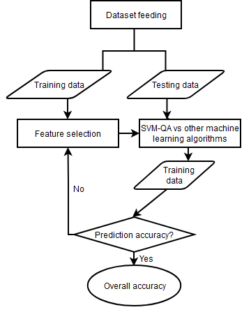
The input dataset is split into a training set and a testing set. This study uses 80% of each input dataset which is a commonly used ratio as the training set and the remaining 20% as the testing set. Since there are variables that do not contribute to the prediction accuracy of the model, and some even reduce the prediction accuracy, recursive feature elimination (RFE) [30] is used to remove such attributes while constructing prediction models. This process is captured in the step feature selection to the training data. The kernel functions of SVM formulated and solved by quantum annealing solvers are used in classifications.

3.3. Evaluation process

To investigate whether quantum machine learning can deliver consistent and reliable results, this study has included two sets of evaluations. In one evaluation, we have selected benchmarks from our own tests using sixteen supervised, semi-supervised, and unsupervised machine learning algorithms. In another test, the benchmarks have been identified from evaluation results of seven traditional machine learning algorithms shared by other researchers on HyberLabelme platform. To improve the generalization of the findings, this study has taken the recommendation of including multiple classifiers for a specific classification task in the evaluation [14-15]. In both rounds of evaluations, only the algorithm that has the best AUROC value for every dataset is identified for that group, and has been used for benchmark purpose. Thus, quantum machine learning is compared against only the best performer for each of the 16 datasets in two rounds of evaluations. This approach would demonstrate whether quantum machine learning delivers consistent results, and having two evaluations has also increased the reliability of the study.

Table 2 has listed all eighteen algorithms used as benchmarks in the two rounds of evaluations. The first set compares the results of SVM-QA with the best results posted on HyperLabelMe using seven classical machine learning algorithms: SVM, random forest (RF), extreme learning machines (ELM), k-nearest neighbor (KNN), linear discriminant analysis (LDA), logistics regression (LR), and fast and deep deformation approximations (FDDA). The results from HyperLabelMe were posted and made available for public access by other researchers. The second set compares the results of SVM-QA with the best results from our own implementation experiments using sixteen out of all eighteen methods listed in Table 2 (excluding Fast and deep deformation approximations and Extreme learning machines used in the first evaluation).

Table 2: Machine Learning Algorithms Used

Python 3.8 and standard packages from the SciKit Learn library are used in coding the 16 classical machine learning algorithms, and D-Wave quantum annealing solver is applied to solve the SVM-QA model.

4. Results

Identification of the optimal γ value is important for the QA module of SVM to achieve good performance in accuracy. To identify the most appropriate one, we have examined the impact of three commonly used γ values (0.125, 0.25, and 0.5) as SVM hyperparameters on the accuracy performance of SVM-QA.

There are primarily two ways to measure the classification accuracy of the models [49]: accuracy and Area Under the Curve of the receiver operating characteristics (AUROC). Accuracy counts how many predictions are correct, whereas AUROC value presents the ratio of true positives to the portion of true negatives (a true positive refers to the case when the model correctly classifies the data, and a true negative occurs when the model correctly identifies the negative class), hence AUROC is more effective in assessing the performance of the models. AUROC has values from 0 to 1, the higher the value, the better the performance. In this study, we use AUROC to measure the performance of the classifiers. The findings indicate that a γ value of 0.125 yields the best accuracy for 10 out of 16 datasets (see Table 3).

Table 3: SVM-QA AUROC with Different γ Settings

The SVM-QA results with the γ value of 0.125 is selected to compare with the best-performing of classical machine learning methods on each of the 16 datasets (see Table 4).

Table 4: SVM-QA vs Best Machine Learning Algorithms

Note: AUROC¹ refers to best result posted on HyperLabelMe using machine learning algorithms, numbered based on their performance: 1-SVM, 2-RF, 3-ELM, 4-KNN, 5-LDA, 6-LR, 7-FDD; AUROC² refers to best results from our tests with 16 machine learning algorithms.

The performance of the classifiers varies depending on the datasets. To evaluate how QML compares to classical machine learning algorithms and produce more generalizable results, Table 4 presents a comparison of accuracy (AUROC) for SVM-QA with the best classifiers as benchmarks in two evaluations. One set of benchmarks is drawn from the results shared by other researchers on HyperLabelMe (column Best * AUROC¹), while the other benchmark datasets are based on our own tests (column Best **AUROC²).

Figure 2 illustrates the AUROCs obtained by applying SVM-QA on the 16 datasets, while Figure 3 shows the AUROC obtained by applying other 16 machine learning algorithms on the Naples95 dataset. D-Wave solver generates a Q matrix out of 80% of the training data and then randomly selects 50 samples from the matrix for training. The hyperparameters for SVM-QA are set as follows: B = 2, K = 2, χ_i = 0, γ = 0.125. Here, B represents the base used for the encoding, K is the number of binary variables used to encode the continuous decision variables, and χ_i is the multiplier for the encoding process. The SVM-QA values are highlighted in bold font when they surpass the results of both other researchers’ tests shared on HyperLabelMe and our tests. In addition, SVM-QA are highlighted in italics when they exceed HyperLabelMe results but are lower than the ones from our tests.

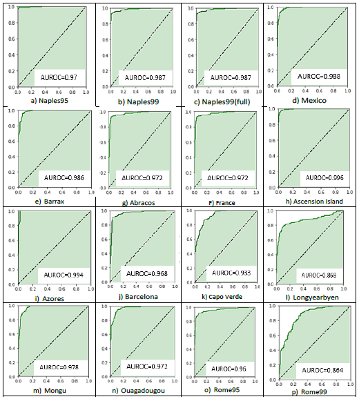
Note: horizontal axis represents false positive rate, and vertical axis represents true positive rate.

Overall, our findings show that SVM-QA provides better accuracy. When compared to both the best results reported on HyperLabelMe and from our own results, SVM-QA performs consistently in classification accuracy, outperforming the reported 7 best machine learning algorithms in 10 out of 16 datasets and comes very close in the remaining datasets.

5. Discussion

Remote sensing data provides information to detect and monitor activities and changes in a geographical area with broad applications in a range of fields [11]. It plays an important role in scientific research areas such as astronomy, oceanic sciences, and atmosphere sciences, as well as commercial applications such as business location selection [50], geolocation-based social networks [51], smart waste collection systems [52], and also social well-being initiatives like poverty alleviation [53].

The rapid growth of remote sensing data collected from various sources has made it imperative to develop and deploy advanced and robust data processing tools. As a result, machine learning and deep learning have been widely used in the classification of remote sensing data. However, the performance of these tools varies depending on the data’s characteristics. In addition, the increasing demand for computing power to develop advanced tools poses a bottleneck for classical machine learning. With quantum computing emerging as a recent technological 

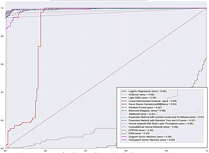
Note: horizontal axis represents false positive rate, and vertical axis represents true positive rate.

breakthrough, offering capabilities for solving computationally impossible complex problems and scaling faster than traditional computing, we are motivated to investigate its potential to overcome the classical machine learning bottleneck in remote sensing image data field.

This study explores how Support Vector Machine, a popular supervised machine learning algorithm, performs when enhanced with quantum annealing. Using 16 labeled and harmonized image datasets from HyperLabelMe, we have compared the classification accuracy of SVM with quantum annealing enhancement to a standard SVM and two sets of top performing classical machine learning algorithms respectively. The results suggest that SVM-QA demonstrates promising accuracy in classification, outperforming most top performing machine learning algorithms that do not have the quantum computing enhancement. Because of quantum computing’s capabilities to improve the performance of classical machine learning algorithms, there has been growing motivation to identify and expand quantum machine learning applications. However, literature on QML’s applications in satellite image classification remains somewhat limited. In [24], the authors report the application of quantum neural network in the satellite image classification and benchmarked it using low-resolution satellite data. Their finding suggests that QML approach produces better results. Studies that have applied other types of data also reach a similar conclusion. For example, in [17], the authors compare the performance of SVM trained on a D-Wave quantum annealer to SVMs used on conventional computers with both synthetic and real biology data, and they find that QML offers more generalizable solutions than the conventional SVM approach.

In this study, we have selected and applied the optimal γ(Gamma) value in the SVM-QA model implemented in the D-Wave computing environment. By comparing its classification results with those of over a dozen best classical machine learning algorithms on 16 HyperLabelMe datasets, our study provides more generalizable findings. This study contributes to the existing literature by offering broader and more in-depth understanding into remote sensing image binary classification. It expands the potential applications of QML in satellite data classification and provides insights into achieving more accurate results.

6. Conclusion

This study has investigated the performance of binary classification of quantum enhanced machine learning algorithm compared to over a dozen classical machine learning algorithms across 16 satellite image datasets. Since support vector machine is a popular machine learning algorithm, we use quantum enhanced SVM in this study. The results suggest that quantum enhanced machine learning approach has often outperformed the classical machine learning approach.

Although SVM-QA has demonstrated superior performance compared to other machine learning algorithms, the evaluation is conducted in the context of harmonized hyperspectral remote sensing image datasets with small sample sizes and binary classification classes. We believe its potential with large datasets waits to be fully explored. We plan to evaluate SVM-QA’s performance on much larger datasets with multiple classification classes and much larger images collected using different types of sensors, such as synthetic aperture radar (SAR) and light detection and ranging (LiDAR).

The development of quantum machine learning has made provision for the escalating development of computing, which will allow the accelerated progress of QML application to solve pressing and practical matters.  Remote sensing is a field that requires multidisciplinary collaborations and inherently demands high computing power. We could leverage QML’s computing capability in conducting real-time remote sensing environmental monitoring, timely disaster response, and efficient resource management. Although still in its infancy, quantum computing will definitely play an indispensable role in the near future.

Conflict of Interest

The authors declare no conflict of interest.

1. S. Cuypers, A. Nascetti, and M. Vergauwen, “Land use and land cover mapping with vhr and multi-temporal sentinel-2 imagery, ” Remote Sensing, vol. 15, 2501, 2023, doi:10.3390/rs15102501.
2. M. Breunig, P.E. Bradley, M.W. Jahn, P.V. Kuper, N. Mazroob, N. R¨osch, M. Al-Doori, E. Stefanakis, and M. Jadidi, “Geospatial data management research: Progress and future directions,” ISPRS International Journal of Geo-Information, vol. 9, no. 95, 2020, doi:10.3390/ijgi9020095.
3. M. Aslam, M.T. Ali, S. Nawaz, S. Shahzadi, and M.A. Fazal, “Classification of Rethinking Hyperspectral Images using 2D and 3D CNN with Channel and Spatial Attention: A Review”, Journal of Engineering Research and Sciences, vol. 2, no. 4, pp. 1-9, 2023, doi: 10.55708/js0204003.
4. Y.D. Pyanylo, V. Sobko, H. Pyanylo, and O. Pyanylo, “ Orthogonal Polynomials in the Problems of Digital Information Processing”, Journal of Engineering Research and Sciences, vol. 2, no. 5, 2023, doi: 10.55708/js0205001
5. Y. Shi, D. Campbell, X. Yu, and H. Li, “Geometry-guided street-view panorama synthesis from satellite imagery,” IEEE Transactions on Pattern Analysis and Machine Intelligence, vol. 44, pp. 10009-10022, 2022, doi:10.1109/TPAMI.2022.3140750.
6. P. Weber and D. Chapman, “Location intelligence: An innovative approach to business location decision-making,” Transactions in GIS, vol. 15, 2011.
7. U. Bayr, “Quantifying historical landscape change with repeat photography: An accuracy assessment of geospatial data obtained through monoplotting,” International Journal of Geographical Information Science, vol. 35, pp. 2026–2046, 2021, doi:10.1080/13658816.2021.1871910.
8. M. Riedel., G. Cavallaro, and J. A. Benediktsson, “Practice and experience in using parallel and scalable machine learning in remote sensing from hpc over cloud to quantum computing,” in 2021 IEEE International Geoscience and Remote Sensing Symposium IGARSS, Brussels, 2021, pp. 1571–1574, doi:10.1109/IGARSS47720.2021.9554656.
9. A. Sebastianelli, D. A. Zaidenberg, D. Spiller, B.L, Saux, and S.L.Ullo, “On circuitbased hybrid quantum neural networks for remote sensing imagery classification,” IEEE Journal of Selected Topics in Applied Earth Observations and Remote Sensing, vol. 15, pp. 565–580, 2021, doi:10.1109/JSTARS.2021.3134785.
10. D.A. Zaidenberg, A. Sebastianelli, D. Spiller, and S.L. Ullo, “Advantages and bottlenecks of quantum machine learning for remote sensing,” in 2021 IEEE International Geoscience and Remote Sensing Symposium IGARSS, Brussels, pp. 5680–5683, 2021, doi:10.1109/IGARSS47720.2021.9553133.
11. G. Cheng, X. Xie, J. Han, L. Guo, and G. Xia, “Remote sensing image scene classification meets deep learning: Challenges, methods, benchmarks, and opportunities,” IEEE Journal of Selected Topics in Applied Earth Observations and Remote Sensing, vol. 13, pp. 3735–3756, 2020.
12. S. Crommelinck, M. Koeva, M.Y. Yang, and G. Vosselman, “Application of Deep Learning for Delineation of Visible Cadastral Boundaries from Remote Sensing Imagery,” Remote Sensing, vol. 11, 2505, 2019, doi: 10.3390/rs11212505.
13. S. Fujita and M. Hatayama, “Estimation method for roof-damaged buildings from aero-photo images during earthquakes using deep learning,” Information Systems Frontiers, vol. 25, pp. 351–363, 2021, doi:10.1007/s10796-021-10124-w.
14. A.E. Maxwell, T.A. Warner, and F. Fang, “Implementation of machine-learning classification in remote sensing: An applied review,” International Journal of Remote Sensing, vol. 39, pp. 2784–2817, 2018, doi:10.1080/01431161.2018.1433343.
15. R. L. Lawrence and C.J. Moran, “The americaview classification methods accuracy comparison project: A rigorous approach for model selection,” Remote Sensing of Environment, vol. 170, pp. 115–120, 2015, doi:https://api.semanticscholar.org/CorpusID:43784543.
16. J. Mu˜noz-Mar´ı, E. Izquierdo-Verdiguier, M. Campos-Taberner, A. P´erez-Suay, L. G´omez-Chova, G. Mateo-Garc´ıa, A.B. Ruescas, V. Laparra, J.A. Padron, J. Amor´os-L´opez, and G. Camps-Valls, “Hyperlabelme: A web platform for benchmarking remote-sensing image classifiers,” IEEE Geoscience and Remote Sensing Magazine, vol. 5, pp. 79–85, 2017, doi:10.1109/MGRS.2017.2762476.
17. D. Willsch, M. Willsch, H. De Raedt, and K. Michielsen, “Support vector machines on the d-wave quantum annealer,” Computer Physics Communications, vol. 248, 107006, 2020, doi:10.1016/j.cpc.2019.107006
18. V. N. Vapnik, The nature of statistical learning theory. In Statistics for Engineering and Information Science, 2000.
19. C. Venkatesan, P. Karthigaikumar, A. Paul, S. Satheeskumaran, and R. Kumar, “Ecg signal preprocessing and svm classifier-based abnormality detection in remote healthcare applications,” IEEE Access, vol. 6, pp. 9767–9773, 2018, doi:10.1109/ACCESS.2018.2794346.
20. H. Cheng, Y. Liu, Y, D. Huang, and B. Liu, “Optimized forecast components-svm based fault diagnosis with applications for wastewater treatment,” IEEE Access, vol. 7, pp. 128534–128543, 2019, doi:10.1109/ACCESS.2019.2939289.
21. K.S. Sahoo, B.K. Tripathy, K. Naik, S. Ramasubbareddy, B. Balusamy, M. Khari, and D. Burgos, “An evolutionary svm model for ddos attack detection in software defined networks,” IEEE Access, vol. 8, pp. 132502–132513, 2020, doi:10.1109/ACCESS.2020.3009733.
22. C.K.I. Williams and M.W. Seeger, “Using the nystr¨om method to speed up kernel machines,” In NIPS, 2000.
23. A. Delilbasic, G. Cavallaro, M. Willsch, F. Melgani, M. Riedel, and K. Michielsen, “Quantum support vector machine algorithms for remote sensing data classification,” in 2021 IEEE International Geoscience and Remote Sensing Symposium IGARSS, pp. 2608–2611, 2021, doi:10.1109/IGARSS47720.2021.9554802.
24. M.P. Henderson, J. Gallina, and M. Brett, “Methods for accelerating geospatial data processing using quantum computers,” Quantum Machine Intelligence, vol. 3, pp. 1–9, 2020, doi:10.1007/s42484-020-00034-6.
25. P. Date, D. Arthur, and L. Pusey-Nazzaro, “Qubo formulations for trainingmachine learning models,” Scientific Reports, vol. 11, 2021, doi:10.1038/s41598-021-89461-4.
26. Kuhn, H., A, W.T.: Nonlinear programming. In: 2nd Berkeley Symposium, pp.481–492, 1951.
27. A. Lucas, “Ising formulations of many np problems,” Frontiers in physics, vol. 2, no. 5, 2014, doi:10.3389/fphy.2014.00005.
28. S. Otgonbaatar and M. Datcu, “Natural embedding of the stokes parameters of polarimetric synthetic aperture radar images in a gate-based quantum computer,” IEEE Transactions on Geoscience and Remote Sensing, vol. 60, pp. 1–8, 2022, doi:10.1109/TGRS.2021.3110056.
29. V.N. Smelyanskiy, E.G. Rieffel, S. Knysh, C.P. Williams, M.W. Johnson, M.C. Thom, W.G. Macready, and K.L. Pudenz, “A near-term quantum computing approach for hard computational problems in space exploration,” arXiv: Quantum Physics, 2012, doi:10.48550/arXiv.1204.2821.
30. I., Guyon, J. Weston, S.D. Barnhill, and V.N. Vapnik, “Gene selection for cancer classification using support vector machines,” Machine Learning, vol. 46, pp. 389–422, 2004. doi:10.1023/A:1012487302797.
31. S.W. Bailey, D. Otte, P.C. DiLorenzo, and J.F. O’Brien, “Fast and deep deformation approximations,” ACM Transactions on Graphics (TOG), vol. 37, pp. 1–12, 2018, doi:10.1145/3197517.3201300.
32. N.S. Altman, “An introduction to kernel and nearest-neighbor nonparametric regression,” The American Statistician, vol. 46, pp. 175–185, 1992, doi:10.2307/2685209.
33. L. Breiman, J..H. Friedman, R. A. Olshen, and C.J. Stone, “Regression Trees,” in Classificationand regression trees, New York, USA, Routledge, 1984, chapter8, doi:10.1201/9781315139470.
34. Y. Freund and R.E. Schapire, “A decision-theoretic generalization of on-line learning and an application to boosting,” Journal of computer and system sciences, vol. 55, no. 1, pp. 119–139, 1997, doi:10.1006/jcss.1997.1504
35. A. Lazarevic and V. Kumar, “Feature bagging for outlier detection,” In Proceedings of the Eleventh ACM SIGKDD International Conference on Knowledge Discovery in Data Mining, 2005, doi:10.1145/1081870.1081891.
36. J.D. Rnnie, L. Shih, J. Teevan, and D.R. Karger, “Tackling the poor assumptions of naive bayes text classifiers,” In Proceedings of the 20th International Conference on Machine Learning (ICML-03), pp. 616–623 2003.
37. A.G. Howard, M. Zhu, B. Chen, D. Kalenichenko, W. Wang, T. Weyand, M. Andreetto, and H. & Adam, “MobileNets: Efficient Convolutional Neural Networks for Mobile Vision Applications,” 2017, ArXiv, abs/1704.04861.
38. Z. Li, Y. Zhao, N. Botta, C. Ionescu, and X. Hu, “Copod: Copula-based outlier detection,” In Proceedings of IEEE International Conference on Data Mining (ICDM), pp. 1118–1123, 2020.
39. M. Pal, “Random forest classifier for remote sensing classification,” International Journal of Remote Sensing, vol. 26, pp. 217–222, 2005 doi:10.1080/01431160412331269698.
40. C. Seiffert, T.M. Khoshgoftaar, J.V. Hulse, and A. Napolitano, “Rusboost: A hybrid approach to alleviating class imbalance,” IEEE transactions on systems, man, and cybernetics-part A: systems and humans, 40, pp. 185–197, 1997. doi:10.1109/TSMCA.2009.2029559.
41. G. Huang, Q. Y. Zhu, and C.K. Siew, “Extreme learning machine: Theory and applications,” Neurocomputing, vol. 70, pp. 489–501, 2006, doi:10.1016/j.neucom.2005.12.126.
42. T. Chen and C. Guestrin, “Xgboost: A scalable tree boosting system,” in Proceedings of the 22nd ACM SIGKDD International Conference on Knowledge Discovery and Data Mining, 2016, doi:10.1145/2939672.2939785
43. A.J. Izenman, “Linear Discriminant Analysis,” In: Modern Multivariate Statistical Techniques, Springer Texts in Statistics, Springer, 2013, New York, NY, doi:10.1007/978-0-387-78189-1_8.
44. G. Ke, Q. Meng, T. Finley, T. Wang, W. Chen, W. Ma, Q. Ye, and T.Y. Liu, “Lightgbm: A highly efficient gradient boosting decision tree,” in Proceedings of the 31st International Conference on Neural Information Processing Systems, Long Beach, pp. 3149–3157, 2017.
45. W. Chen, Y. Chen, Y. Mao, and B.L. Guo, “Density-based logistic regression,” in Proceedings of the 19th ACM SIGKDD International Conference on Knowledge Discovery and Data Mining, 2013, doi:10.1145/2487575.2487583
46. S. Lee and J.Y. Choeh, “Predicting the helpfulness of online reviews using multilayer perceptron neural networks,” Expert Systems with Applications, vol. 41, pp. 3041–3046, 2014, doi:10.1016/j.eswa.2013.10.034.
47. C.J. Burges, “A Tutorial on Support Vector Machines for Pattern Recognition,” Data Mining and Knowledge Discovery, vol. 2, pp. 121-167. 1998.
48. P. H. Chen, C.J. Lin, and B. Sch¨olkopf, “A tutorial on v-support vector machines”, Applied Stochastic Models in Business and Industry, vol. 21, pp. 111–136, 1997, doi:10.1002/asmb.537.
49. J.A. Hanley and B.J. McNeil, “The meaning and use of the area under a receiver operating characteristic (roc) curve,” Radiology, vol.143, no. 1, pp. 29–36, 1982, doi:10.1023/A:1012487302797.
50. Y. Xu, Y. Shen, Y. Zhu and J. Yu, “Ar2net: An attentive neural approach for business location selection with satellite data and urban data,” ACM Transactions on Knowledge Discovery from Data, vol. 14, no. 2, 20, pp. 1-28, 2020, doi:10.1145/3372406.
51. A. Likhyani and S.J., P, D. Bedathur, “Location-specific influence quantification in location-based social networks,” ACM Transactions on Intelligent Systems and Technology (TIST), vol. 10, pp. 1–28, 2019. doi:10.1145/3300199.
52. J.M. Gutierrez, M. Jensen, M. Henius, and T.M. Riaz, “Smart waste collection system based on location intelligence,” vol. 61, pp. 120–127, 2015, doi:10.1016/j.procs.2015.09.170.
53. N. Jean, M., Burke, S.M. Xie, W.M. Davis, D. Lobell, and S. Ermon, “Combining satellite imagery and machine learning to predict poverty,” Science, vol. 353, pp. 790–794, 2016, doi:10.1126/science.aaf7894.

Citations by Dimensions

Citations by PlumX

Crossref Citations

This paper is currently not cited.

No. of Downloads per Month

No. of Downloads per Country