Robust and accurate localization is crucial for mobile robot navigation in complex indoor environments. This paper introduces a robust and integrated robot localization algorithm designed for such environments. The proposed algorithm, named Branch-and-Bound for Robust Localization (BB-RL), introduces an innovative approach that seamlessly integrates global localization, position tracking, and resolution of the kidnapped robot problem into a single, comprehensive framework. The process of global localization in BB-RL involves a two-stage matching approach, moving from a broad to a more detailed analysis. This method combines a branch-and-bound algorithm with an iterative nearest point algorithm, allowing for an accurate initial estimation of the robot’s position. For ongoing position tracking, BB-RL uses a local map-based scan matching technique. To address inaccuracies that accumulate over time in the local maps, the algorithm creates a pose graph which helps in loop-closure optimization. Additionally, to make loop-closure detection less computationally intensive, the branch-and-bound algorithm is used to speed up finding loop constraints. A key feature of BB-RL is its Finite State Machine (FSM)-based relocalization judgment method, which is designed to quickly identify and resolve the kidnapped robot problem. This enhances the reliability of the localization process. BB-RL’s performance was thoroughly tested in real-world situations using commercially available logistics robots. These tests showed that BB-RL is fast, accurate, and robust, making it a practical solution for indoor robot localization.

1. Introduction

The growing demand for mobile robots in tasks such as repair, transportation, and cleaning necessitates the development of efficient techniques for robot localization [1]–[5]. Particularly in known environments, robots should be able to localize themselves within a prebuilt map, enabling them to position themselves based on data collected from various sensors. The problem of localizing mobile robots in indoor environments can be categorized into three sub-problems: position tracking, global localization, and the kidnapped robot problem [6, 7]. This paper proposes a fast, robust, and accurate algorithm to achieve indoor localization of mobile robots, effectively solving the three localization sub- problems simultaneously in real-world applications.

Recent advancements in indoor robot localization re- search have shown significant progress, yet challenges remain in simultaneously addressing three critical localization issues. The first issue involves global localization. Often, an initial pose is determined by observing the robot’s approximate position in the environment to reduce computational effort and maintain localization stability. Despite this, without an initial estimate, achieving desirable global localization remains difficult.

The second issue is position tracking. Here, the challenge lies in the timely elimination of accumulated errors. To address this, two main strategies are employed. The first is simultaneous localization and mapping (SLAM), which involves frontend scan matching and backend optimization. While effective, SLAM methods are computationally demanding and rely on loop-closure detection to correct errors. The second strategy involves odometry, such as visual or LiDAR odometry, which calculates the robot’s relative pose incrementally using adjacent data. However, these methods are prone to error accumulation over time, making them suitable primarily for short-term tracking.

Finally, the third issue is the kidnapped robot problem. This occurs when a robot, initially well-localized, is unexpectedly moved to an unknown location. This problem can be split into two scenarios: real kidnapping, where the robot is physically relocated by external forces such as human intervention or an accident, and perceived kidnap- ping, which results from localization failures. Addressing this issue effectively remains a challenge for most existing approaches.

Considering these aspects, we propose a robust and accurate robot localization algorithm, which consists of three parts: global localization, position tracking, and relocalization judgment.

• The global localization algorithm, which is used to determine the robot’s initial pose, can be divided into two stages. In the coarse matching stage, the branch-and- bound algorithm based on depth-first search (DFS) is used to promptly identify the absolute position of the robot on the map without any initial In the fine matching stage, the iterative nearest point algorithm is used to perform iterative optimization to determine the optimal initial pose of the robot. This algorithm can rapidly converge anywhere on the map, and the robot pose exhibits global optimality.
• The position tracking algorithm is used for the continuous localization of the robot when the initial pose is A local map-based scan matching method is used to estimate the relative pose of the robot and simultaneously build a local map. Moreover, a global pose graph optimization algorithm is used to eliminate the accumulated errors between local maps. Additionally, to ensure that the computing time is nonintractable, a DFS-based branch-and-bound algorithm is used to accelerate the process of identifying the loop constraints.
• The relocalization judgment algorithm is used to address the problem of robot kidnapping and eliminate the accumulated errors of the robot. We propose an FSM-based relocalization judgment method based on confidence calculation and dual-threshold judgment to effectively monitor the localization status of the robot. When the calculated confidence is less than the minimum threshold, the global localization algorithm is invoked for localization recovery.

The main contributions of this research can be summarized as follows:

1. Development of a Two-Stage Global Localization Algorithm: We introduce a novel two-stage global localization algorithm that combines the broad search capabilities of the branch-and-bound algorithm with the local optimization efficiency of the iterative closest point algorithm. This ensures the robot quickly identifies the globally optimal initial pose without relying on any preliminary estimates.
2. Establishment of a Position Tracking Algorithm: Our re- search incorporates a position tracking algorithm that integrates frontend local map-based scan matching with backend pose graph This approach provides a highly accurate state estimation of the robot, crucial for precise navigation.
3. Creation of an FSM-based Relocalization Judgment Algorithm: We have developed an innovative FSM-based relocalization judgment algorithm that utilizes an inflated occupancy grid map to minimize the impact of sensor measurement noise. This algorithm is adept at efficiently detecting instances of robot kidnapping, thereby safeguarding against localization failures in diverse scenarios and ensuring swift and effective localization recovery.

4. Proposal of a Joint Localization Algorithm: The research culminates in a comprehensive joint localization algorithm capable of concurrently addressing the challenges of global localization, position tracking, and robot kidnapping in indoor settings. The efficacy of this algorithm has been rigorously validated using commercial logistics robots, demonstrating its successful application in real-world environments.

2. Related work

Consistent and efficient localization is a core concept of in- door robot navigation, as knowledge of the robot position is crucial in deciding future actions [8]. In recent years, several researchers have focused on indoor robot localization [9]. However, most of the existing approaches focus on solving a specific problem of localization (such as global localization), which is fundamentally different from the motivation of our work.

Localization refers to the procedure of determining the robot pose with respect to its environment by using various noisy sensors. According to the type of measurement data, the sensors used in the process of robot localization can be divided into two classes: proprioceptive sensors and exteroceptive sensors. Proprioceptive sensors (such as encoders and IMUs) measure the robot motion by using deduced reckoning to calculate the relative robot displacement [10]– [12]. Since such sensors consider the instantaneous speed or acceleration to estimate the robot state, the integrated error in the localization process increases in a nonbounded manner over time. Hence, such sensors are usually used in combination with exteroceptive sensors that can determine the absolute positions to enhance the robot’s ability in managing uncertainties [13]–[16]. Proprioceptive sensors address position tracking issues due to their inability to sense environmental information.

In addition to the methods based on proprioceptive sensors for localization, several approaches use exteroceptive sensors to recognize the environment around a robot to estimate the robot location. Among these methods, SLAM is widely used. In terms of the primary type of adopted sensor, the SLAM algorithm can be divided into two classes: visual SLAM and LiDAR SLAM. Visual SLAM aims to address the pose estimation of cameras with visual information. This method has evolved from the use of monocular cameras [17] to stereo cameras [18] and depth cameras [19]. The classic variants of monocular SLAM include ORB-SLAM [20], DSO [21], LSD-SLAM [22], and SVO [23]. Certain researchers, [24] adapted ORB-SLAM to a fisheye camera, tightly coupled visual information and IMU data to robustly estimate the camera pose and used the multimap technology to effectively solve the problem of localization failure. In another study [25], a rolling- shutter camera and IMU were tightly coupled to minimize the photometric error to estimate the robot pose. Other researchers [26, 27, 28] used deep neural networks to eliminate the scale ambiguity of monocular cameras and extract high-level semantic features to enhance the system robust- ness and accuracy. The classic variants of stereo SLAM include ORBSLAM2 [29], ORBSLAM3 [30], PL-SLAM [31], and SOFT2 [32]. An event camera [33] was used to address the problems of high dynamics and low light, and the depth estimation of multiple viewpoints was merged in a probabilistic manner to build a semidense point cloud map. Notable research on RGB-D SLAM includes that on the RTAB-MAP [34], bundle fusion [35], and Kintinuous [36]. Moreover, a lightweight semantic network model was pro- posed [37], which integrates multiple technologies such as VIO, pose graph optimization, and semantic segmentation, to achieve the high-precision reconstruction of the three- dimensional environment. Deep learning techniques have also been employed in visual SLAM to extract features, enhancing the algorithm’s ability to interpret and understand the visual information as in LIFT-SLAM [38] and Object- Fusion [39]. Because depth cameras can directly obtain the depth information of the environment, their use has been widely considered [40]. However, processing of the depth data is computationally expensive, and it is difficult to satisfy the real-time operation requirements of the CPU. Moreover, the frontend odometry aspects of visual SLAM can only estimate the relative pose of the robot, and back- end loop-closure detection can only achieve relocalization in similar scenes. Therefore, this approach cannot realize global localization.

LiDAR SLAM can be divided into 2D LiDAR SLAM and 3D LiDAR SLAM according to the type of LiDAR used. The classic 3D LiDAR SLAM algorithms include LOAM [41], HDL graph slam [42], and SuMa++ [43]. LOAM exhibits a high performance on the KITTI dataset, and thus, many improved versions of this algorithm have been proposed. In [44], the distinctive edge features and planar features were extracted to achieve two-step Levenberg–Marquardt optimization. In [45], the LiDAR and IMU data were tightly coupled. The IMU preintegration factor was introduced in the pose graph optimization to update the bias of the IMU, and the accumulated errors were corrected through loop-closure detection. Moreover, excellent schemes for 2D LiDAR SLAM have been proposed in recent years. The classic filter-based algorithms include Fast SLAM [46] and Gmapping [47], and graph-based algorithms include Karto SLAM [48] and Cartographer [49]. Cartographer, developed by Google engineers, has been proven to be a complete SLAM system that integrates localization, mapping, and loop-closure detection. At the frontend of this algorithm, the relative pose of the robot is calculated using the scan- to-submap matching method, which has a significantly lower accumulated error than the scan-to-scan matching method [50]. Additionally, compared with the scan-to-map matching method [51], it is considerably less computation- ally intensive and can run in real time. Similarly, since the origin of the robot localization is determined when initializing the algorithm, LiDAR SLAM is essentially an odometry technique and cannot solve the problems of global localization and robot kidnapping. To realize indoor localization, 2D LiDAR has been widely used due to its cost and accuracy. Certain researchers [52] and [53] attempted to enhance the accuracy of their localization system by using the extended Kalman filter to achieve multisensor fusion. However, these approaches cannot solve the problems of global localization and robot kidnapping. In [54], a quasistandardized 2D dynamic time warping (QS-2DDTW) method was proposed to solve the problem of robot kidnapping. The approach uses scan data for two consecutive ranges to obtain the geometric shape similarity of the environment to determine the robot state. Nevertheless, this approach cannot solve the position tracking problem. However, other studies [55]–[59] addressed the three major localization problems by using the adaptive Monte Carlo localization algorithm. Notably, using only ultrasonic sensors, the localization accuracy of the order of decimeters can be achieved.

In addition to the two types of exteroceptive sensors for localization, several wireless devices (such as WiFi, UWB, Bluetooth, and RFID) can be deployed indoors to realize reliable localization. In [60] and [61], the Kalman filter was used to fuse IMU and UWB data to obtain a relatively accurate robot pose. However, these approaches could not solve the problems of global localization and robot kidnapping. In addition, high accuracy localization was achieved using commercial WiFi devices [62]. The robust principal component analysis for extreme learning machine algorithm (RPCA-ELM) could suppress the effect of measurement noise in the localization process. In [63] and [64], to enhance the robustness of localization, UHF radio frequency identification technology was adopted. However, the system accuracy depended on the RFID tag, and global localization could not be realized at arbitrary positions. Furthermore, localization was realized in [65] and [66] by deploying a set of photoresistor sensors on a robot to collect information regarding an LED array in the environment. However, high-precision position tracking could not be realized. In addition, a robot localization system based on asynchronous millimeter-wave radar interference was proposed [67], which used the interference between multiple millimeter-wave radars with known positions in the environment to calculate the position of the robot. However, the system exhibited limited localization accuracy.

In summarizing the state of the art in indoor robot localization, it is clear that researchers have made significant strides using a variety of methodologies and sensor technologies. From SLAM implementations—both visual and LiDAR-based—to sophisticated sensor fusion techniques leveraging proprioceptive and exteroceptive sensors, including the use of wireless technologies like WiFi, UWB, Bluetooth, and RFID to enhance localization capabilities, each method aims to address specific facets of the complex challenge of localization, focusing on global localization, position tracking, or resolving the kidnapped robot problem.

Despite these advances, a comprehensive solution that simultaneously addresses all three critical challenges of indoor robot localization remains elusive. Existing studies tend to focus on optimizing specific aspects of localization rather than offering a unified algorithm capable of handling global localization, precise position tracking, and the kidnapped robot scenario in an integrated manner. This gap in the research landscape underscores the innovative potential of the proposed BB-RL algorithm, which aims to provide a holistic approach to the multifaceted problem of autonomous indoor navigation. By doing so, BB-RL aspires to establish a new method in the field, offering a more ro- bust, accurate, and comprehensive solution to indoor robot localization than currently available methods.

Some literature mentions studies that attempt to address all three major localization challenges simultaneously using the Adaptive Monte Carlo Localization algorithm [55]–[59]. These studies illustrate the potential of multi-sensor fusion and intelligent algorithms to enhance indoor localization accuracy and robustness. However, despite offering a composite solution, these approaches may still face limitations in practical application, such as dependency on specific types of sensors, the impact of environmental complexity on localization accuracy, and challenges in maintaining high precision in dynamic and unknown environments.

The Self-Adaptive Monte Carlo Localization (SA-MCL) method represents an advancement in addressing the inherent challenges of robot localization, including global localization, position tracking, and the “kidnapping” problem, where a robot is moved to an unknown location. Previous studies have shown that by employing the adaptive Monte Carlo localization algorithm, significant strides can be made in solving these three major localization challenges. These methods, however, are predominantly based on 2D environments and utilize ultrasonic sensors for sensing.

Transitioning from 2D to 3D environments introduces new challenges for the Monte Carlo Localization (MCL) algorithm. In [68], the authors propose a pure 3D MCL localization algorithm to address these challenges directly. Meanwhile, other approaches, such as the one by [69], adapt 2D MCL for localization in 3D maps. These methods illustrate the diversity of strategies being explored to solve localization problems in three-dimensional spaces using the MCL framework in 3D Map. The demand for computational resources and memory usage significantly increases in 3D Monte Carlo localization due to the necessity to process and track a much larger number of particles to accurately estimate a robot’s pose in three-dimensional space. Each particle’s position, orientation, and weight must be maintained, leading to escalated memory requirements as the particle count increases. Furthermore, without prior knowledge of the robot’s approximate location, distributing particles effectively throughout the three-dimensional space to ensure comprehensive coverage and, by extension, the accuracy of the localization process, presents a considerable challenge. This challenge underscores the complexity of initializing the algorithm in 3D spaces, which is vital for the successful application of Monte Carlo localization methods in more complex environments.

In [70], the authors developed a branch-and-bound (BnB)-based 2D scan matching technique utilizing hierarchical occupancy grid maps of varying sizes. While this approach provides accurate and fast global localization on 2D maps, its processing time significantly increases when applied to 3D maps. In [71], the authors advanced this research by introducing a BnB-based method for 3D global localization, which more effectively addresses the challenges of extending the work of [70] to three-dimensional environments. However, these studies primarily focus on global localization issues without offering an integrated solution. In summary, despite attempts to address the three major localization challenges simultaneously and the existence of various methods focusing on solving specific issues, there remains a significant research gap in developing an accurate and robust comprehensive localization system. This high- lights the importance and innovative value of proposing new algorithms, such as the BB-RL algorithm introduced in this paper, aimed at enhancing the performance of indoor robot localization. The BB-RL algorithm seeks to overcome the limitations of existing solutions through innovative techniques and methods, providing a more comprehensive and effective solution to meet the demands of complex indoor environments for robot navigation.

3. System overview

3.1. Hardware setting

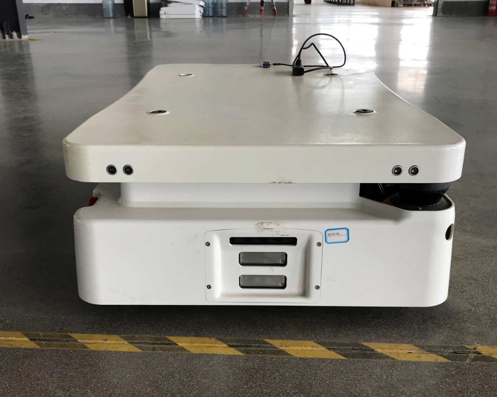
The hardware settings are shown in Figure 1. The adopted autonomous mobile robot (AMR) is a commercial differential wheeled logistics robot, model IR300, which is equipped with an Intel NUC8BEH minicomputer as the computing platform of the robot; two SICK TIM561 LiDAR for range measurements, which are deployed diagonally on the left front and bottom right of the robot and have a measurement frequency of up to 10 Hz; an inertial measurement unit model LMPS-be1, which is used for high-frequency linear acceleration and angular velocity measurement and can exhibit a measurement frequency of up to 200 Hz; two wheel encoders, which are used to measure the wheel speed with a measurement frequency of up to 50 Hz.

3.2. System architecture

The system architecture of the proposed algorithm is shown in Figure 2. The algorithm is composed of three parts: global localization, position tracking, and relocalization judgment.

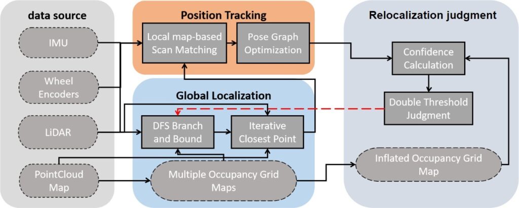
In the localization process, we first obtain the robot’s initial pose in the environment through the global localization algorithm, which is a two-stage matching algorithm composed of a branch-and-bound algorithm and an iterative closest point algorithm. After determining the robot’s initial pose, we implement the position tracking algorithm, which uses the initial pose as the robot’s initial state to realize local map-based scan matching. To effectively eliminate the accumulated errors between local maps, we maintain a global pose graph at the backend of the algorithm. When a valid loop closure is detected, the algorithm is implemented to correct the accumulated errors. Finally, we use a single thread to implement the relocalization judgment algorithm to monitor whether the robot can be located correctly when the position tracking algorithm is used. When the confidence of the current localization result is less than the set dual-thresholds, the global localization algorithm is called to reinitialize the algorithm.

4.  Global Localization

Global localization, as an indispensable part of our algorithm, is mainly used to determine the robot’s initial pose and ensure localization recovery when the robot is kid- napped. When the algorithm is implemented, we first con- vert the prebuilt point cloud map into multiple occupancy grid maps with different resolutions. Subsequently, we use the DFS-based branch-and-bound algorithm to accelerate the matching of the current LiDAR data with the occupancy grid maps. Finally, the iterative nearest point algorithm is used to continue the optimization on the computational results of the DFS-based branch-and-bound algorithm and ensure rapid convergence to obtain the optimal pose of the robot.

4.1. Global search using the branch-and-bound algorithm

We formulate global localization as a search problem on the occupancy grid map. The linear and angular search window sizes can be easily determined according to the map size. To ensure the search accuracy, we set the linear step size as the grid size. The angular step size can ensure that the farthest LiDAR point s_max moves once without exceeding the map resolution r. Thus, the angular step size ε can be estimated using the following equation:

$$\varepsilon \, \arccos\left(1 – \frac{r^2}{2s_{\text{max}}^2}\right) \tag{1}$$

Furthermore, the integral number of steps covering the set linear and angular search window sizes can be computed as:

$$s_x \left\lfloor \frac{S_x}{r} \right\rfloor, \; s_y \left\lfloor \frac{S_y}{r} \right\rfloor, \; s_\theta \left\lfloor \frac{S_\theta}{\varepsilon} \right\rfloor \tag{2}$$

where S _x and S _y are the linear search window sizes in the x- and y-directions, respectively. S _θ is the angular search window size. s_x and s_y are the integral numbers of the linear steps in the x- and y-directions, respectively, and s_θ is the integral number of the angular steps. If the center of the occupancy grid map is assumed to be the origin of the search process, the search set can be defined as:

$$\mathbf{W} = \left\{-\frac{1}{2}s_x, \ldots, \frac{1}{2}s_x \right\} \times \left\{-\frac{1}{2}s_y, \ldots, \frac{1}{2}s_y \right\} \times \left\{-\frac{1}{2}s_\theta, \ldots, \frac{1}{2}s_\theta \right\} \tag{3}$$

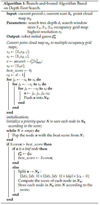
Because the time to search an occupancy grid map in- creases exponentially with increasing map size, we apply the branch-and-bound algorithm to accelerate the search process. In practical applications, we build a global search tree to determine the initial pose for a given occupancy grid map, where each node in the tree represents a search result. The map search process is converted into node transversal in the search tree, and the target is to identify the leaf node with the best score.

In contrast to the breadth-first search-based branch-and- bound algorithm, which traverses most of the nodes in the search tree to identify the leaf node with the best score, we use the DFS-based branch-and-bound algorithm to promptly evaluate the nodes by performing a layer-by-layer search on multiple occupancy grid maps with low to high resolutions and prune the intermediate nodes that do not meet the boundary conditions and all the corresponding subnodes. Therefore, only a few nodes need to be traversed to identify a leaf node with the best score. The flow of the algorithm is illustrated in Figure 3.

Schematic of the DFS-based Branch-and-Bound Method (Search Tree Depth d 3). The root node is implicitly divided into different subnodes to form a set N₀, and a node n₀ is extracted to illustrate the algorithmic process.

First, we use the prebuilt point cloud map to create multiple occupancy grid maps with high to low resolutions. Specifically, we first rasterize the point cloud map according to the required highest resolution r₀. The probability value of each grid is averaged according to the number of point clouds in the grid, and the resulting occupancy grid map is denoted as map₀. Subsequently, according to the depth d of the global search tree, map₀ is downsampled d − 1 times. The resolution of map_ii 1, …, d − 1 obtained by each downsampling is doubled to 2ⁱr₀. Finally, we save these maps from low to high resolutions.

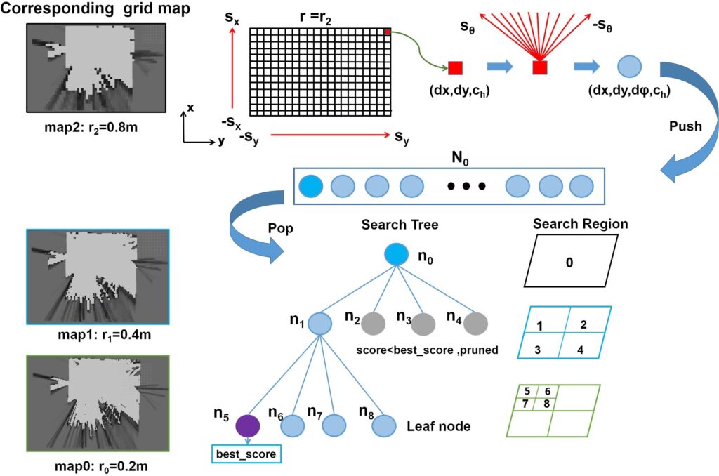
Second, we consider the search strategy. In the global search tree, the root node corresponds to the set of all possible solutions. We do not explicitly express this node but only branch it into a series of child nodes, which can be denoted as the set N0 of all possible solutions searched on map_d−1. The leaf nodes represent a possible solution searched on map₀. Each node n_i in the tree is represented as a tuple of integers:

$$\mathbf{n}_i \quad dx, dy, d\varphi, c_h \tag{4}$$

where dx and dy represent the position offsets in the x and y directions relative to the origin of the search process, respectively. dφ is the rotation offset relative to the positive direction of the search process, and c_h represents the height of the search tree in which the node is located. Each node in the search tree is defined as a search area with a certain boundary.

Each node with c_h > 1 can branch into four child nodes of height c_h − 1:

$$N_n \ \{2dx, 2dx, 1\} \times \{2dy, 2dy, 1\} \times \{d\varphi\} \times \{c_h – 1\} \tag{5}$$

For each leaf node with c_h 0, branching cannot continue to generate new nodes. Thus, the search pose corresponding to the leaf node is a possible solution. When the leaf node with the best score is found, the optimal solution to the problem can be expressed as

$$\xi_n^* \quad ro\,dx,\,ro\,dy,\,\varepsilon d\varphi \tag{6}$$

Finally, the upper bound calculation strategy is implemented. An excellent upper bound can help promptly identify the optimal solution to the problem. To ensure the accuracy of the upper bound, when building multiple occupancy grid maps with low to high resolutions, the probability value of each grid in map_ii 1, …, d − 1 is the maximum probability value of the corresponding 2ⁱ × 2ⁱ grids in map₀. Therefore, the grids on the occupancy grid map with a lower resolution have a higher probability value:

$$Score_n \quad \sum_{i1}^{N} F_{Multimap}^{C_h} T_{\xi_n} S_i \tag{7}$$

where F^ch_Multimap transforms the LiDAR point to the map frame to obtain the probability of the corresponding grid according to the prebuilt multiple occupancy grid maps. The search process is essentially a table lookup process, and thus, the computational complexity of the algorithm is always maintained in a constant range. The specific steps of the algorithm are shown in Algorithm 1.

 4.2. Optimization of the initial pose using the iterative nearest point algorithm

Although the pose ξ^∗_n specified by the DFS-based branch- and-bound algorithm has global optimality, the final search accuracy is inevitably limited by the highest resolution of the occupancy grid map. Hence, we use the iterative closest point algorithm to further optimize ξ^∗_n.

The iterative nearest point algorithm calculates the rigid transformation matrix between the two sets of point clouds in an iterative manner. We convert the matching problem between the two sets of point clouds into a nonlinear least squares problem and iteratively compute the rigid transformation matrix around the initial value ξ^∗_n We assume that the robot pose in the iterative process is ξ x, y, φ, the point in the point cloud map is p′_i , the current LiDAR point is p_i, and the error function e is defined as

$$e^{\xi} \arg\min \frac{1}{2} \sum_{i1}^{N} \left\| p_i – \exp^{\hat{\xi}} p_i’ \right\|_2^2 \tag{8}$$

where exp· represents the exponential mapping of so3 → S O3. We can use iterative algorithms (e.g., Gauss–Newton and Levenberg–Marquardt) to solve this problem. The Jacobian matrix of the iterative update process can be expressed as follows:

$$\frac{\partial e}{\partial \delta \xi} – I \exp^{\hat{\xi}} \hat{p}_i \tag{9}$$

The convergence speed of the iterative nearest point algorithm is affected by the maximum number of iterations and the robot pose difference calculated by two consecutive iterations. When the algorithm is used on hardware-constrained robot platforms, and it is necessary to consider the operating efficiency and localization accuracy, the convergence conditions can be alleviated. Our algorithm provides a satisfactory initial guess. Additionally, the number of point clouds involved in the matching is small. Hence, the con- vergence condition can be met after several iterations.

5. Position Tracking

The position tracking algorithm is of significance in enhancing the performance of the localization algorithm, especially in challenging circumstances such as those involving map expiration or environmental changes due to dynamic obstacles. In this paper, we use a scan matching method that aligns the current LiDAR data with the local map. The local map contains a certain number of LiDAR frames, which are expressed in an occupancy grid map. The map is updated continuously with each new LiDAR data. When the local map is built, it is added to the backend pose graph for optimization. The accumulated errors are corrected with the introduction of loop constraints to ensure the accuracy of the position tracking algorithm.

5.1. Frontend local map-based scan matching

The matching process involves inserting the current LiDAR data into the appropriate position in the local map. We formulate this process as a local nonlinear optimization problem, in which the LiDAR pose is optimized relative to the current local map. The problem is solved using the Gauss–Newton method. By iteratively optimizing the error function, a LiDAR pose with the highest probability is identified. In the optimization problem, T_ξ denotes the transformation matrix that transforms the LiDAR data into the local map. The error function can be expressed as:

$$E\xi \, \arg\min_{i1}^{N} \left(1 – FT_{\xi} s_i\right)^2 \tag{10}$$

where F : R₂ → R represents a bicubic interpolation function that smooths the sum of the probability values of each LiDAR point in the local map. Specifically, we assume that T_{ξ s} is defined as a point x, y in the two-dimensional plane. In this case, the bicubic interpolation function is:

$$F_{x,y} = \sum_{i=0}^{3} \sum_{j=0}^{3} f_{x_i,y_j} W_{x – x_i} W_{y – y_j} \tag{11}$$

where f x_i, y _j is the probability of the four neighborhoods x_i, y _j around the point x, y, and W· represents the weight of the x_i, y _j interpolation on x, y, computed as:

$$W_x = \begin{cases} a(2|x|^3 – 3|x|^2 + 1) & \text{for } |x| \leq 1 \\ a|x|^3 – 5a|x|^2 + 8a|x| – 4a & \text{for } 1 < |x| < 2 \\ 0 & \text{otherwise} \end{cases} \tag{12}$$

where a takes values in the range −0.75, −0.5. Solving Eξ is a local nonlinear optimization problem. Thus, a satisfactory initial guess is critical. Before scan matching, we use a two-stage pose prediction method to obtain this initial guess. First, we use the extended Kalman filter (EKF) algorithm to fuse the wheel odometry and IMU data. The process uses these two types of data as observation information to update the state of the moment, as in [12].

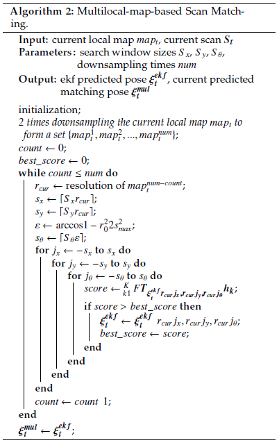
Second, we use a multilocal-map-based scan matching method to further optimize the fusion result. The specific process is shown in Algorithm 2.

In the beginning, we perform a 2× downsampling on the local map to generate multiple local maps with resolutions ranging from high to low. Subsequently, we intend to find a LiDAR pose that maximizes the probabilities at the current LiDAR data in the lowest resolution local map. The initial pose is provided by the fusion result. Moreover, to ensure the matching accuracy, the pose obtained by matching against this local map is used as the initial value of the subsequent matching. This process is repeated until the matching against the highest resolution local map is realized, and the optimal initial guess is obtained.

After identifying the appropriate position, we insert the LiDAR data into the local map. This process updates the probability value of the corresponding grid. Each insertion of the LiDAR data is equivalent to adding an observation, and the result of the observation is saved using a hit set and miss set. According to the ray-tracing model, we use the projected LiDAR point as the hit point and save the grid point closest to this hit point in the hit set. Each grid point passing through the rays between the hit point and LiDAR data origin is saved in the miss set.

When the grid in the local map has never been observed previously, the probability is zero. When the grid is observed for the first time, it is assigned a probability value determined by its set (hit set or miss set). Each subsequent observation is based on the following formula to update the probability value of the grid:

$$S \ S^{-} \ \textit{LogMeas} \tag{13}$$

where S is the probability value of grid s after observation z, S ⁻ is the probability value of grid s before observation, and LogMeas represents the measurement model of the up- date process, which can be defined as

$$S \ \textit{logOdds} \mid z \tag{14}$$

$$S^{-} \ \textit{logOdds} \ \log \frac{ps \cdot 1}{ps \cdot 0} \tag{15}$$

$$\textit{LogMeas} \ \log \frac{pz \mid s \cdot 1}{pz \mid s \cdot 0}, \ z \in \{0, 1\} \tag{16}$$

where the logOdd function converts the product operation between the probability values into an addition operation, ps 1 is the probability that grid s is occupied before the observation, and ps 0 is the probability that grid s is free before the observation. According to the value of z, LogMeas has two states. The specific value is determined by the sensor characteristics.

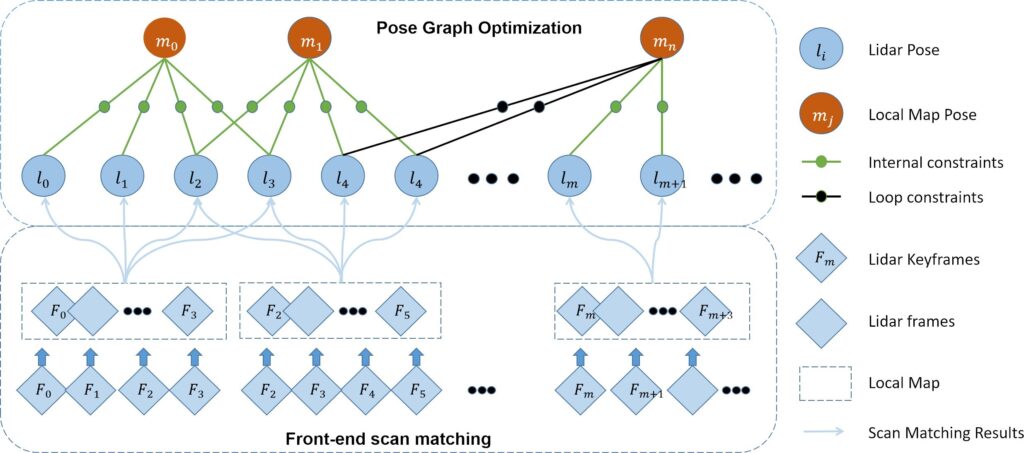
5.2. Backend pose graph optimization

The local map-based scan matching method can only decrease the short-term accumulated errors. However, the built local maps also accumulate errors over time, which can be optimized by building a global pose graph in the backend. In this process, we first use LiDAR frames that satisfy both rotation and translation conditions as key frames. Subsequently, we add all the keyframes and local maps to the pose graph as nodes to be optimized. Finally, the estimated trajectory is smoothed according to the constraints between the keyframe nodes and local map nodes. The optimization process of the pose graph is shown in Figure 4.

After a newloop constraint is constructed in the backend of the algorithm, we optimize the pose graph. We formulate the optimization process as a nonlinear least squares problem, in which the error term describes the error between the measured and estimated values. We consider the keyframe i and local map j as examples. The pose of keyframe i in the world frame is ξ^s_i , and the pose of local map j in the world frame is ξ^l_j. The error term can be expressed as

$$e_{ij} \ z_{ij} – h(\xi_{i}^{s}, \xi_{j}^{l}) \tag{17}$$

where zi j is the relative pose measured between keyframe i and local map j, calculated through loop-closure detection. hξ^s_i , ξ^l_j is the relative pose estimated between keyframe i and local map j, which represents the result of the local map-based scan matching.

generated by keyframes and local maps that have subordination relationships. Specifically, the keyframes are inserted in the local map. In contrast, the loop constraints are generated by keyframes and other local maps, that is, the keyframes are associated with historical local maps. When more local maps are added to the pose graph, the time to identify the loop constraints gradually increases. Therefore, a DFS- based branch-and-bound algorithm is used to accelerate the search for loop constraints.

The process of loop-closure detection is similar to that of the DFS-based branch-and-bound algorithm used in global localization, except that the search range is changed from a global map to historical local maps. Hence, the search window no longer contains the prebuilt map but a partial area inside the local map. Because the frontend provides the current pose estimation ξ _{f ront} of the robot, we use the pose as the search origin to traverse the search space around it. The result ξ_loop is defined as 

$$\xi_{loop} \ \xi_{front} \ r_0 dx, r_0 dy, \varepsilon d\varphi \tag{18}$$

If k represents the constraint between local map i and keyframe j, the error function can be expressed as

$$\arg\min_{k1}^{K} \, \mathbf{e}_k^{T} \xi_k^{es}, \xi_k^{l} \mathbf{\Sigma}_k^{-1} \mathbf{e}_k \xi_k^{es}, \xi_k^{l} \tag{19}$$

where Σ⁻¹_k is the information matrix of the error term formed by keyframe i and local map j. The objective of optimizing the error function is to adjust ξ^s and ξ^l to minimize the trajectory errors formed by all nodes. Since no constraint relationship exists between each local map and keyframe in the pose graph, in solving the nonlinear optimization problem, considerable time is not required to calculate the Hessian matrix and only the pose increment needs to be solved via the Cholesky decomposition.

6. Relocalization judgment

In numerous practical application scenarios, such as in ware- house logistics, robots are required to accomplish specific tasks within extensive workspaces. Due to the inability to form loop closures within short periods, robots tend to accumulate errors gradually. Furthermore, challenges arise when incorrect observational data leads to ’robot kidnap- ping’, making it arduous to achieve localization recovery solely through position tracking algorithms.

In light of these challenges, we introduce an FSM (Finite State Machine)-based relocalization judgment algorithm. This algorithm initiates by acquiring the confidence level of the robot’s current pose through the alignment of current LiDAR data with an inflated occupancy grid map. Subsequently, based on pre-set dual-threshold conditions, we assess the necessity to engage the global localization
algorithm for timely localization recovery.

6.1. Confidence calculation and dual-threshold judgment

We use a method similar to the calculation of scores in scan matching to verify the pose ξ_pt obtained by the position tracking algorithm. In contrast to the point cloud registration algorithm that adopts the Euclidean distance to calculate the matching score between the two point clouds, we use the pose ξ_pt to project the current LiDAR data S onto the occupancy grid map and calculate the sum of the probability values of each LiDAR point s_i falling on the corresponding grid:

$$Score_{\xi_{pt}} = \frac{1}{N} \sum_{i1}^{N} MT_{\xi_{pt}} s_i \tag{20}$$

where T_ξpt converts the current LiDAR data S from the LiDAR frame to the map frame, and M· is used to calculate the probability value of each LiDAR point projected onto the occupancy grid map.

In this process, the occupancy grid map is converted from the prebuilt point cloud map. The resolution of this map is the same as that of the local map generated by the position tracking algorithm.

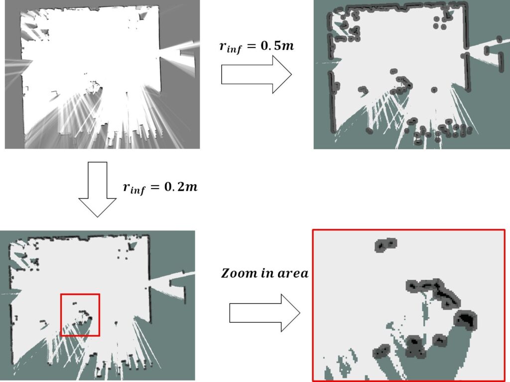
In practical applications, since there are relatively few valid points in the LiDAR frame, the measurement error of each valid point affects the confidence calculation results Considering this aspect, we use an inflated occupancy grid map instead of the original occupancy grid map to suppress the impact of LiDAR measurement errors.

In contrast to the cost map used to set the expansion areas to avoid robot collisions, we use the inflated occupancy grid map to reduce the error caused by noisy LiDAR measurements. When designing the inflated occupancy grid map, we first set the expansion radius r_{in f} according to the sensor range accuracy and extend it outward from the obstacle to obtain the expansion area according to r_{in f} . The grid probability in the expanded area is 

$$P_{inf, x, y} = e^{-k \delta d} \tag{21}$$

where δd is the distance between grid x, y and the obstacle, and k is the scale factor. When k is large, the grid probability P_{in f}  x, y decreases rapidly. The probability of P_{in f}  x, y is limited to the range 0, 1. The process of generating an inflated occupancy grid map is shown in Figure 5. We update the confidence calculation formula as follows:

$$Score_{\xi_{pt}} = \frac{1}{N} \sum_{i=1}^{N} M^{InfMap} T_{\xi_{pt}} s_i \tag{22}$$

formula, we use the dual-threshold judgment to evaluate the pose ξ_pt.

1. When the confidence is greater than the set threshold T_h2, the LiDAR data are projected inside the expansion area of the map, and the errors of the confidence calculation are generated by the noisy LiDAR measurements,
2. When the confidence is between the two thresholds T_h1 and T_h2 T_h2 > T_h1, the accumulated errors exceed expectations, and the robot kidnapping problem does not occur. Therefore, we call the global localization algorithm to complete the search in the local area near the pose ξ_pt to correct the accumulated errors.
3. When the confidence is less than the set threshold T_h1, the robot kidnapping problem is considered to We invoke the global localization algorithm to search the whole map. Specifically, the search window of the branch-and-bound algorithm covers the occupancy grid map to complete the localization recovery.

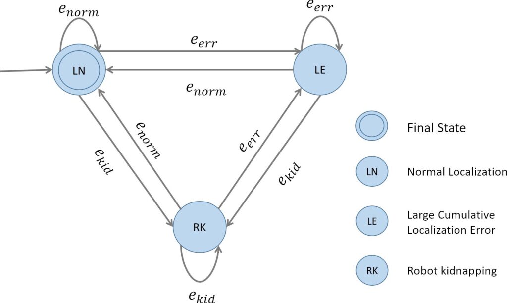
6.2. Relocalization judgment based on finite state machine

To monitor the localization state in real time, we use the idea of a finite state machine to model the relocalization judgment process. The mathematical model for a certain finite state machine can be defined as

$$M = \langle Q, \Sigma, \delta, q_0, F \rangle \tag{23}$$

where Q is a nonempty set consisting of a finite number of states. According to the results of the position tracking algorithm, the states of the whole algorithm are divided into three categories: normal localization q_norm, large localization error q_err, and localization failure q_kid, which correspond to three cases of the dual-threshold judgment. Therefore, Q can be defined as

$$\mathbf{Q} = \{ q_{norm}, q_{err}, q_{kid} \} \tag{24}$$

where Σ represents the set of all inputs that can be accepted by each state, that is, the set of trigger conditions that cause the state transition. In this algorithm, we use the result of the dual-threshold judgment as the trigger condition. Additionally, we use e_norm, e_err and e_kid to represent the inputs of the algorithm in the transition between q_norm, q_err and q_kid. At this time, Σ is defined as

$$\Sigma = \{ e_{norm}, e_{err}, e_{kid} \} \tag{25}$$

where δ : Q × Σ → Q represents the state transition function, which is mainly based on the current trigger condition e to complete the state transition of the algorithm from the current state q_cur to the second state q_sec:

$$q_{sec} \;\delta q_{cur},\; e \tag{26}$$

where q₀ is the initial state. F is the set of termination states, which is a subset of Q that represents that the algorithm is acceptable in this state (for instance, q_norm).

At the beginning of the algorithm operation, the robot is normally located. We first define the initial state q₀ as the state q_norm and subsequently determine the trigger condition according to the result of the confidence calculation.

1. If the result of the confidence calculation is greater than T_h2, the condition e_norm is triggered. The algorithm maintains the state q_norm and outputs the result of the position tracking algorithm.
2. When the result of the confidence calculation is between T_h1 and T_h2 T_h2 > T_h1, the condition e_err is triggered. The algorithm executes the function δq_norm, e_err to achieve the transition from q_norm to q_err, that is, the global localization algorithm is called to perform a search in the local range.
3. When the result of the confidence calculation is less than T_h1, the condition e_kid is triggered. The algorithm executes the function δq_norm, e_kid for the transition be- tween the two states of q_norm to q_kid. Specifically, the global localization algorithm is invoked to perform a search on the global map.

The state transition relationship in the finite state machine is shown in Figure 6. The specific steps of the FSM- based relocalization judgment algorithm are shown in Algorithm 3.

This algorithm is expected to solve the problem of robot kidnapping. Hence, it is necessary to search for the best matches on the global map. To ensure the stability of the algorithm, we limit the number of calls to the global localization algorithm to manage the errors in the confidence calculation caused by environmental changes (such as dynamic environments). Our confidence calculation method averages the matching probabilities of each LiDAR point participating in the scan matching. The method exhibits a certain degree of robustness in scenarios involving slight environmental changes; however, its performance is limited in cases involving severe environmental changes. Thus, it is preferable to limit the number of calls to global localization. When the set maximum number of times is reached, the relocalization judgment algorithm is automatically terminated.

7. Experiments

As described in this section, we validate the robustness and accuracy of our algorithm through extensive experiments. First, we present the implementation details, including the experimental environment and preparation steps. Second, we describe the evaluation of our algorithm in a simulated laboratory environment and analysis of the performance of different parts. Finally, we assess the performance of our algorithm in an actual workshop environment.

7.1. Implementation Details

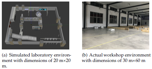
Using the Gazebo physical simulation platform, we build a virtual laboratory environment that mimics the layout and dimensions of the real-world laboratory. In such a typical structured environment, we use a simulated jackal robot with basic sensors (e.g., 2D LiDAR, IMU, and wheel encoders) to perform the experiments. To perform the assessment in an actual workshop environment, we use the IR300 commercial logistics robot to conduct the experiments. The environments are shown in Figure 7(a) and Figure 7(b). In the preparation stage, we use an open-source 2D Li- DAR SLAM algorithm to build a point cloud map of the environment. The process can be divided into three stages:

1. Data preprocessing: Raw sensor data for time synchronization are collected to alleviate the errors caused by the difference in the working frequency of different sensors;
2. Mapping: The handle is used to ensure that the robot can traverse the complete environment to build a point cloud map in real time;
3. Postprocessing: The built point cloud map is filtered to eliminate anomalies and outliers.

7.2. Localization experiment in the simulated laboratory environment

We first test the global localization in the simulated laboratory environment. The size of the laboratory is approximately 20 m×20 m; thus, we set the linear search window sizes in the x- and y-directions as 30 m, respectively, and the angular search window size is set as 2π. The depth of the search tree in the branch-and-bound algorithm is 7. Correspondingly, there exist seven built occupancy grid maps, in which the highest resolution of the occupancy grid map is r₀ 0.4 To ensure that the iterative nearest point algorithm can achieve the highest accuracy, we set the maximum number of iterations as 100 and maximum tolerance of two consecutive iterations as 10⁻¹³.

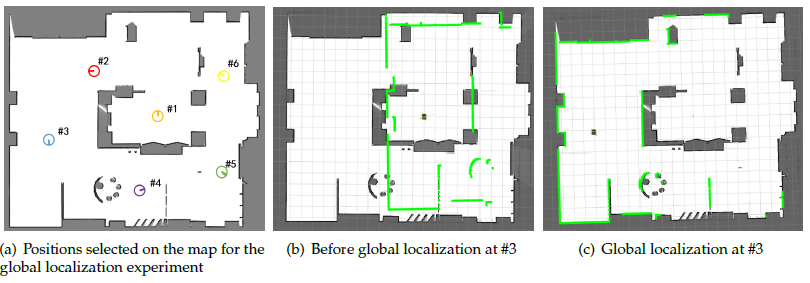
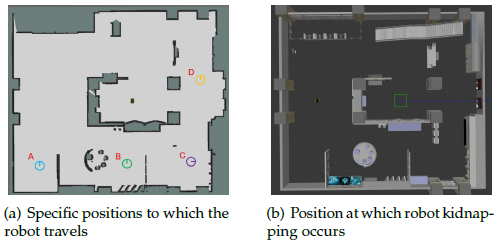
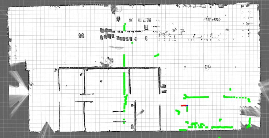
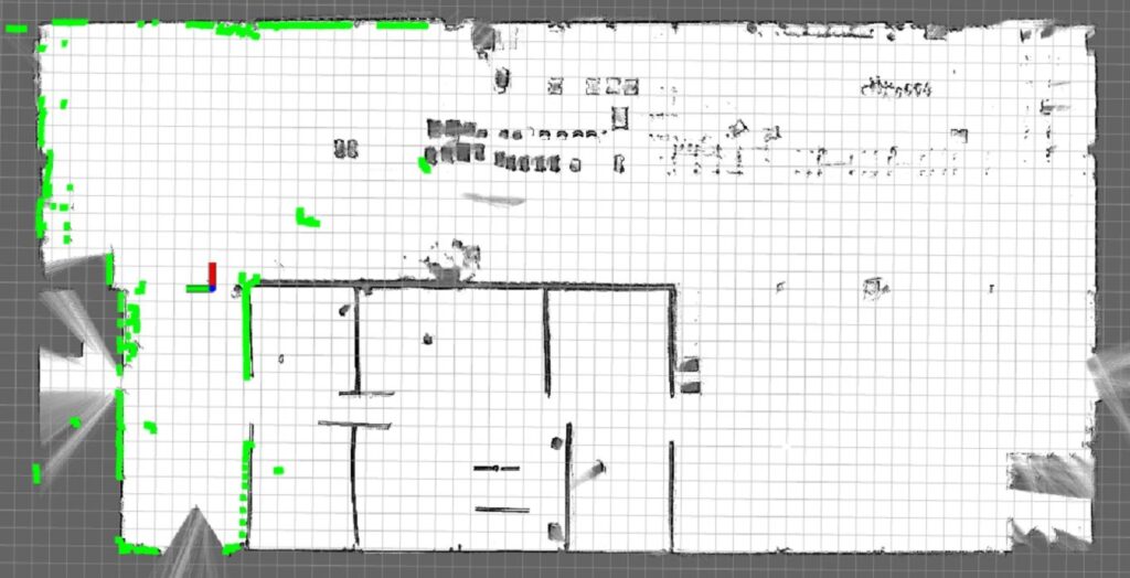
In the experiment, we select six positions on the map to test the performance of the algorithm. To uniformly cover the free space of the environment, the selected adjacent positions are separated by ∆d 5 m, and the orientations of each position are uniformly distributed in −π, π, as shown in Figure 8(a). When the robot starts operating, it automatically implements the global localization algorithm to obtain the robot’s initial pose based on the current LiDAR data, as shown in Figure 8(b) and Figure 8(c).

e_x and e_y denote the position error between the real position and estimated position of the robot, and e_φ represents the difference between the real and estimated orientations. In addition to these standard criteria, we consider the run- time and success rate of the algorithm. The runtime refers to the time from the beginning of the algorithm to the time at which the final result is obtained. The success rate describes the probability of successful localization at the specified position. When the error between the real position and estimated position of the robot is less than 0.05 m and the orientation error is less than 2^◦, the localization is considered successful. We perform 20 experiments for each specified position.

In the test, we verify the performance of the proposed algorithm. Hence, a comparison experiment is not conducted for the following reasons:

1. The localization result is compared with the real position of the robot;
2. Few open-source algorithms can achieve global localization. Actual results for the few algorithms that can accomplish this function have been extensively reported. Therefore, the details do not need to be

According to Table 1, the average orientation error is less than 0.2^◦, the average position errors in the x- and y-directions are less than 0.03 m and 0.01 m, respectively. As described in Section 4, the search accuracy of the branch- and-bound algorithm is limited by the highest resolution of the occupancy grid map (0.4 m). However, the two-stage matching algorithm achieves a localization accuracy that is higher than that of algorithms that use an occupancy grid map with a resolution of 0.05 m for scan matching. Moreover, we achieve a 100% localization success rate in each position.

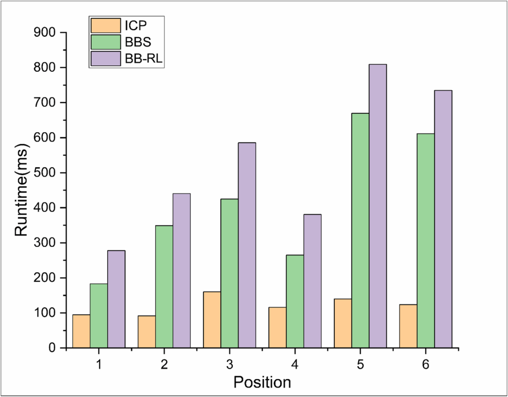
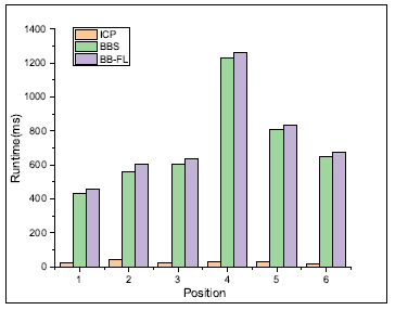
The runtime varies considerably across positions (Figure 9). According to the runtime of each stage in the global localization algorithm, the most notable time consumption pertains to the determination of the initial pose by the branch-and-bound algorithm. In contrast, the runtime of the iterative closest point algorithm is stable and occupies only a small proportion. Although the runtime does not meet the requirements of real-time localization, considering the actual size of the map used in the search process, our algorithm can promptly find the global pose of the robot and dramatically decrease the time associated with redundant calculations.

In the algorithm, when the depth (d 7) is constant, the resolution r₀ of map₀ used in the branch-and-bound algorithm directly influences the localization accuracy and runtime. We analyze the impact of the different resolutions r₀ on the algorithm at position 4 −6.33, 1.23, −45^◦. The results are shown in Table 2. When r₀ is small, although the solution obtained by the branch-and-bound algorithm is closer to the optimal solution, the search time is large. In contrast, the proposed algorithm achieves a reasonable balance between the efficiency and localization accuracy. The localization result obtained by the proposed algorithm does not considerably fluctuate with the change in r₀, and the runtime is exponentially decreased.

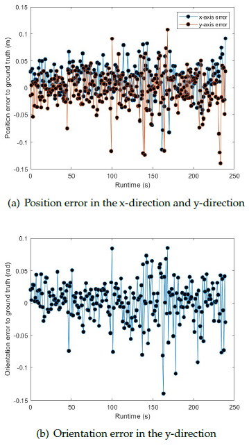
To assess the accuracy of our algorithm, we conducted 50 experimental runs in the simulation environment, and for each run, we randomly selected a position on the map to measure the error. The results are shown in Figure 10. The average position errors in the x- and y-directions are 0.02037 m and 0.00648 m, respectively. The average orientation error is 0.00129 rad, and the average runtime is 576.35 ms. Additionally, the maximum position error in the x- and y-directions are 0.0317 m and 0.0185 m, respectively. The maximum orientation error is 0.00353 rad, and the maximum runtime is 1027.67 ms.

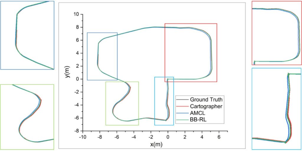
Next, we conduct the position tracking experiment. We assume that the robot’s initial pose is known (automatically obtained by Gazebo). In the test, the robot moves in a circle around the indoor environment. The starting and ending points coincide. We evaluate the error of the robot between the starting and ending points. The process is shown in Figure 11. As a reference, we compare the AMCL and Cartographer frameworks to verify the accuracy of the algorithm.

In the parameter settings, the number of local maps for multi-local-map-based scan matching was established as 3. For loop-closure detection, the linear search window size was set at 20 m and the angular search window size for loop detection at 2π radians. Additionally, the search depth was defined as 7.

The trajectory of each algorithm is shown in Figure 12.

Table 1: Global localization results for specific positions in the simulated laboratory environment.

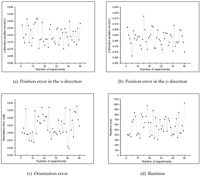
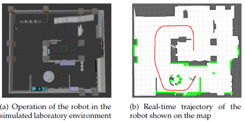
Table 2: Experimental results of global localization algorithm at position 4 with different resolutions r₀.

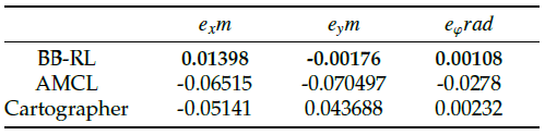
Results obtained using AMCL, Cartographer, and the pro- posed algorithm are relatively close to the ground truth because the sensor data obtained in the simulation environment are ideal, and no sensor failures or other emergencies occur. However, according to the analysis of trajectory de- tails, the proposed algorithm fits the ground truth more closely. According to the trajectory error comparison shown in Table 3, the proposed algorithm outperforms the com- pared algorithms in terms of the accuracy. The Figure 13 shows the time-based error of the position on both the x- axis and y-axis, as well as the orientation error during the position tracking experiment.

Finally, the relocalization experiment is conducted. Since the correction of the accumulated errors is reflected in the experimental results of the position tracking, we test only the localization recovery ability of the algorithm in the case of robot kidnapping. First, we initialize the robot and control it to move in the environment. Second, we suddenly move the robot to positions A, B, C, and D (Figure 14) to artificially create a robot kidnapping situation to verify the effectiveness of the relocalization. Due to only a few existing open-source algorithms can solve the robot kidnapping problem. Additionally, no uniform standard for the ex- perimental procedure exists. Hence, we do not conduct a comparison experiment in this test.

Table 3: Comparison of the position tracking error in the simulated laboratory environment.

Before the test, to ensure that the map has the same resolution as that of the local map used in the position tracking algorithm, we convert the prebuilt point cloud map into an occupancy grid map with a resolution of 0.05 m. According to the range accuracy of the LiDAR, the expansion radius r_{in f} is set as 0.1 m, the scale factor is set as 1, and the thresholds T_h1 and T_h2 are set as 0.5 and 0.8. The experimental results are shown in Figure 15.

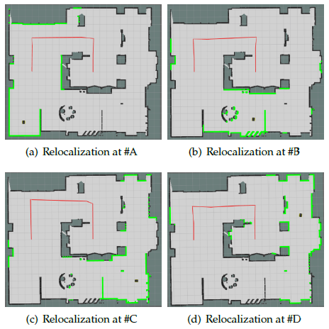
The quantitative results are shown in Table 4. Among these results, the average position errors in the x- and y- directions are less than 0.03 m and 0.01 m, respectively, the orientation error is less than 0.1^◦, the runtime is within 600 ms, and the success rate at each position is consistent with global localization, remaining at 100%. From the overall perspective, the relocalization results are similar to those of the global localization in the simulation environment. When the relocalization judge algorithm is used to identify if the robot is kidnapped, localization recovery can be effectively realized by calling the global localization algorithm.

7.3. Localization experiment in the actual workshop environment

A global localization experiment is conducted in the actual workshop environment. In this experiment, the parameters of the branch-and-bound algorithm are changed. Because the size of the workshop is approximately 60 m ×30 m, we set the linear search window sizes in the x- and y-directions as 70 m and 40 m, respectively. All other parameter settings are the same as those in the global localization experiment in the simulated laboratory environment.

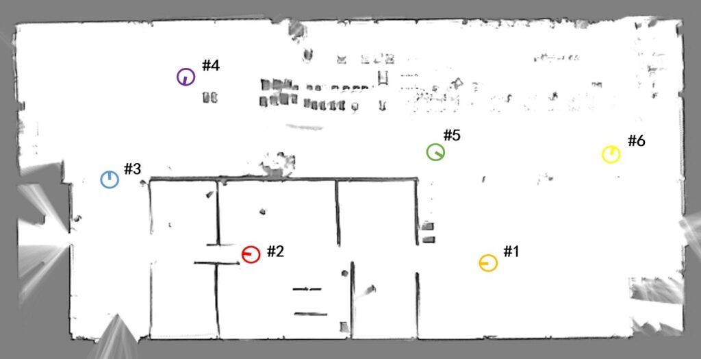
Similarly, we select six positions on the map to analyze the performance of the algorithm. Each adjacent position is separated by ∆d 15 m, and the orientation of each position is uniformly distributed in −π, π. The selected positions are shown in Figure 16. The localization process of position 3 is shown in Figure 17 and Figure 18. The evaluation criteria and number of experiments are the same as those in the global localization experiment in the simulated laboratory environment.

According to Table 5, the average position errors in the x- and y-directions are less than 0.032 m and 0.02 m, respectively, and the average orientation error is less than 1.2^◦. Compared with the experimental results of global localization in the simulated laboratory environment, the error of global localization in the workshop environment is significantly larger. The sensor noise and interference of the dynamic environment in the actual environment are more

Table 4: Relocalization results for specific positions in the simulated laboratory environment.

unpredictable than those in the simulation environment and directly affect the localization accuracy.

The success rate is slightly decreased at positions 3-6 be- cause the current LiDAR data tend to produce mismatches with the occupancy grid map. The runtime associated with each stage in the global localization algorithm (Figure 19) shows that the overall runtime at each position increases. Especially, at position 4, the overall running time is 1260.87 ms, 1226.81 ms of which correspond to the branch-and-bound algorithm. This finding demonstrates that most of the time consumed by the global localization algorithm pertains to the branch-and-bound algorithm implementation.

Moreover, in this experiment, we test the impact of different resolutions r₀ of map₀ used in the branch-and-bound algorithm on the localization accuracy and runtime when the depth (d 7) remains unchanged. The experimental results at position 1 −0.43, −0.365, 0^◦ are shown in Table 6. Compared with the results of the simulated laboratory environment, the runtime at different resolutions r₀ is higher due to the increased size of map₀. However, the proposed algorithm exhibits similar localization accuracies at different resolutions r₀. Therefore, we can choose r₀ 0.4 m to balance localization efficiency and accuracy.

Table 6: Experimental results of global localization algorithm at position 1 with different resolutions r₀.

To assess the accuracy of the global localization algorithm, we conducted 50 experiments in a real-world environment. For each experiment, we randomly selected a position on the map to evaluate the error. The results are shown in Figure 20. The average position errors in the x- and y-directions are 0.02516 m and 0.0079 m, respectively. The average orientation error is 0.0089 rad, and the average runtime is 734.18 ms. Additionally, the maximum position errors in the x- and y-directions are 0.03675 m and 0.02669 m, respectively. The maximum orientation error is 0.0193 rad, and the maximum runtime is 1407.48 ms. Compared with the results in the simulated laboratory environment, the position error and runtime are higher, although the actual engineering needs can still be satisfied.

Next, we perform the position tracking experiment. First, we assume that the robot’s initial pose is the origin of the map in this experiment. Subsequently, we control the robot to move in a circular path in the workshop to return to the starting point. Finally, the error between the starting point and ending point is calculated as the accuracy criterion. As a reference, we compare the results of EKF fused with IMU and wheel odometry, AMCL, and Cartographer to verify the accuracy of the algorithm. The experiment is shown in Figure 21 and Figure 22 .

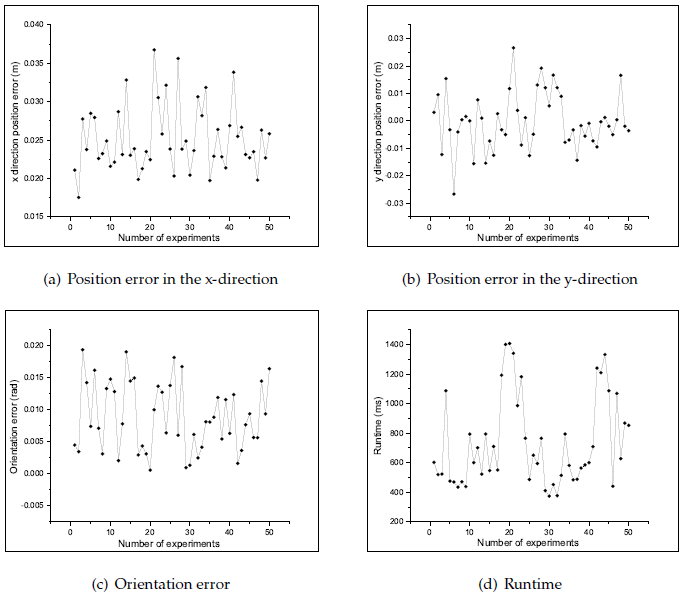
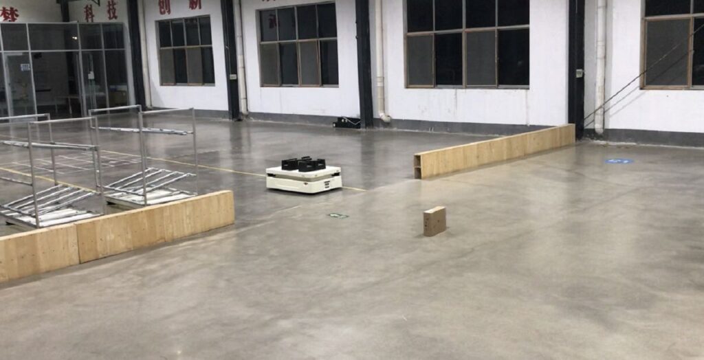
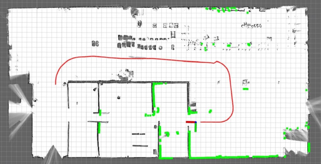
Figure 22: Real-time trajectory of the robot shown on the map in the actual workshop environment.

All the parameter settings are the same as those in the position tracking experiment in the simulated laboratory environment. The trajectory of each algorithm is shown in Figure 23. Notably, (1) the trajectory error associated with the EKF fusion is the largest; (2) there exists a certain deviation in the local details between each trajectory; and (3) the trajectory of the AMCL near the starting point is not closed.

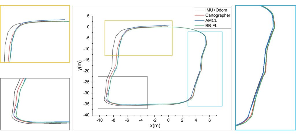
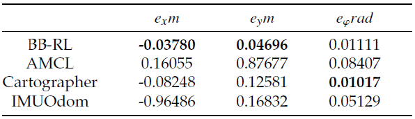
According to Table 7, the position error in the x-direction of EKF fusion is approximately 1 m, the position error in the y-direction of AMCL is approximately 0.9 m, and the orientation error of AMCL exceeds 4.5^◦. In contrast, the proposed algorithm achieves satisfactory results in all aspects: the position errors in the x- and y-directions are both less than 0.05 m, and the orientation error is less than 1^◦.

Table 7: Comparison of position tracking errors in the actual workshop environment.

Finally, a relocalization experiment is conducted in the

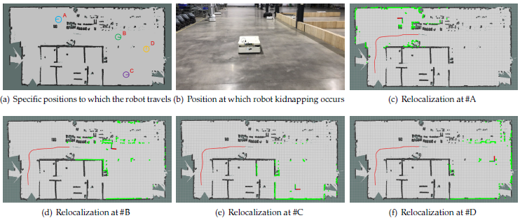
Table 8: Relocalization results for specific positions in the actual workshop environment.

actual workshop environment. The same experimental method as that of the relocalization experiment in the simulated laboratory environment is followed: First, the robot is controlled to move in the workshop through the handle. Second, a robot kidnapping situation is created by artificially moving the robot to positions A, B, C, and D (Figure 24(a) and Figure 24(b)). Finally, the position error and orientation error of different positions are calculated. In terms of the parameter settings, the thresholds T_h1 and T_h2 are set as 0.5 and 0.75, respectively. The resolution of the inflated occupancy grid map is 0.05 m, the expansion radius r_{in f} is set as 0.2 m, and the scale factor k is set as 1. The experimental results are shown in Figure 24(c), Figure 24(d), Figure 24(e) and Figure 24(f).

According to Table 8, the error in the actual workshop environment is higher than that in the simulated laboratory environment. At position A, the position error in the x- direction exceeds 0.028 m, the orientation error exceeds 0.2^◦, and the runtime is close to 1 s. Additionally, the runtime at positions C and D is significantly decreased with values of only 374.754 ms and 434.718 ms, respectively. For the success rate, relocalization failures occur at positions A and B.However, overall, the success rate is maintained at each selected position.

Building on the introduction of the Branch-and-Bound for Robust Localization (BB-RL) algorithm, the experimental findings can be effectively summarized. The BB-RL algorithm offers a potent solution for indoor robot localization by harmoniously integrating position tracking, global localization, and the resolution of the kidnapped robot dilemma within a cohesive framework. The evaluation shows that BB-RL achieves a balance among speed, accuracy, and robustness, establishing it as an effective and practical choice for indoor robot localization scenarios.

In summary, the proposed trajectory aligns more closely with the ground truth compared to those generated by other compared algorithms. The BB-RL algorithm surpasses competing algorithms in accuracy. Regarding the kidnapping problem, robots equipped with BB-RL successfully overcome localization failures, maintaining a commendable success rate. The effectiveness of the BB-RL algorithm in solving the three core localization challenges has been con- firmed in real-world settings, achieving sustained accuracy and an appropriate execution frequency. This underscores the algorithm’s viability and efficiency in practical applications, particularly in navigating and localizing within indoor environments.

8. Conclusion and Future Work

A robust and accurate localization is crucial for effective path planning, precise motion control, and reliable obstacle avoidance in the field of autonomous robotics. Recognizing the need for accurate and robust localization in real-world applications, this paper presents a BB-RL (Branch-and-Bound for Robust Localization) algorithm for indoor mobile robots. Its novelty lies in the comprehensive and integrated approach to addressing the three key localization tasks: global localization, position tracking, and the kidnapped robot problem.

The approach begins with a two-stage global localization algorithm to determine the robot’s initial pose. A DFS-based branch-and-bound algorithm ensures the search solution is globally optimal. To achieve localization precision beyond grid resolution, the iterative closest point (ICP) algorithm refines this solution locally.

For continuous position tracking, a local map-based scan matching technique is used. To achieve reliable results, a two-tier prediction method combining an Extended Kalman Filter (EKF) with multi-local map-based scan matching is proposed, ensuring initial guesses converge to the global optimum. Additionally, a global pose graph is constructed to minimize accumulated errors across local maps, while a DFS-based branch-and-bound algorithm accelerates loop- closure detection.

Long-term stability of the algorithm is maintained through an innovative Finite State Machine (FSM)-based relocalization judgment method, which uses an inflated occupancy grid map to reduce LiDAR measurement noise effects on confidence calculations. A dual-threshold judgment strategy accurately identifies the robot’s localization state, triggering the global localization algorithm as needed for timely localization recovery.

In conclusion, our algorithm shows out for its robust- ness, scalability, and practicality, underscored by its fast processing capabilities. Extensively tested in both simulated laboratory environments and real-world workshops, it has also been successfully implemented on a commercial logistics robot platform. This deployment demonstrates not only its high localization accuracy but also its robust and rapid performance in diverse operational contexts.

Finally, we have underscored the advantages of our localization framework, especially in indoor environments prone to localization difficulties, such as logistics warehouses and factory inspections. These environments require a robust and accurate localization algorithm. By integrating existing sensor data with advanced algorithms, our framework significantly improves localization accuracy and robustness in these complex scenarios.

In the future, our research will focus on utilizing a broader array of features for robot localization, including the features from 3D point cloud maps and camera sensors. These data types promise to enhance localization accuracy by providing a richer set of environmental information. However, incorporating these algorithms and features is expected to increase computational demands. A key direction for our future work will be to find a balance between integrating these diverse and multi-dimensional features and maintaining efficient processing speeds. We aim to integrate 3D point cloud features for improved relocalization without compromising computational efficiency.

Another aspect of our future work will address the challenges posed by complex, dynamic environments, such as scenarios where robots are surrounded by crowds. Identifying the cause of localization failures—whether due to actual kidnapping scenarios or temporary disruptions caused by dynamic environmental factors—and deciding whether to initiate relocalization presents a challenge we plan to address. This involves differentiating between true kidnapping situations and temporary conditions caused by dynamic environments, thereby guiding the decision on whether relocalization is necessary.

This comprehensive approach, leveraging a variety of data sources and technologies, is designed to ensure that localization challenges, even in the most demanding environments, can be effectively addressed. Our goal is to provide a more comprehensive and reliable solution for indoor robot localization, overcoming current limitations and preparing for future challenges.

Conflict of Interest The authors declare no conflict of interest.

1. DeSouza, Guilherme N and Kak, Avinash C, “Vision for mobile robot navigation: A survey”, IEEE transactions on pattern analysis and machine intelligence, vol. 24, no. 2, pp. 237–267, 2002.
2. Georgiev, Atanas and Allen, Peter K, “Localization methods for a mobile robot in urban environments”, IEEE Transactions on Robotics, vol. 20, no. 5, 851–864, 2004.
3. Alatise, Mary B and Hancke, Gerhard P, “A review on challenges of au- tonomous mobile robot and sensor fusion methods”, IEEE Access, vol. 8, pp. 39830–39846,
4. Altan, Aytac¸ and Bayraktar, Ko¨ ksal and Hacıog˘ lu, Rıfat, “Simultaneous localization and mapping of mines with unmanned aerial vehicle”, 2016 24th Signal Processing and Communication Application Conference (SIU), 1433–1436, 2016, doi:10.1109/SIU.2016.7496019.
5. Aytac¸ Altan and Rıfat Hacıog˘ lu, “Model predictive control of three-axis gimbal system mounted on uav for real-time target tracking under external disturbances”, Mechanical Systems and Signal Processing, vol. 138, p. 106548, 2020, doi:https://doi.org/10.1016/j.ymssp.2019.106548.
6. Cox, Ingemar Johansson and Wilfong, Gordon Thomas, Autonomous robot vehicles, Springer, Schweiz, 1990.
7. Thrun, Sebastian and Beetz, Michael and Bennewitz, Maren and Burgard, Wolfram and Cremers, Armin B and Dellaert, Frank and Fox, Dieter and Haehnel, Dirk and Rosenberg, Chuck and Roy, Nicholas and others, “Probabilistic algorithms and the interactive museum tour-guide robot minerva”, The international journal of robotics research, 19, no. 11, pp. 972–999, 2000.
8. Alqahtani, Ebtesam J and Alshamrani, Fatimah H and Syed, Hajra F and Alhaidari, Fahd A, “Survey on algorithms and techniques for indoor navigation systems.”, 2018 21st Saudi Computer Society National Computer Conference (NCC), pp. 1–9, 2018, doi:10.1109/NCG.2018.8593096.
9. Zafari, Faheem and Gkelias, Athanasios and Leung, Kin K, “A survey of indoor localization systems and technologies”, IEEE Communications Surveys & Tutorials, vol. 21, no. 3, pp. 2568–2599, 2019, doi: 1109/COMST.2019.2911558.
10. Liu, Wenxin and Caruso, David and Ilg, Eddy and Dong, Jing and Mourikis, Anastasios I and Daniilidis, Kostas and Kumar, Vijay and Engel, Jakob, “Tlio: Tight learned inertial odometry”, IEEE Robotics and Automation Letters, 5, no. 4, pp. 5653–5660, 2020, doi:10.1109/LRA.2020.3007421.
11. Brossard, Martin and Bonnabel, Silvere, “Learning wheel odometry and imu errors for localization”, 2019 International Conference on Robotics and Automation (ICRA), 291–297, 2019, doi:10.1109/ICRA.2019.8794237.
12. Moore, Thomas and Stouch, Daniel, “Intelligent autonomous systems 13”, 335–348, Springer, Padua, 2016, doi:10.1007/978-3-319-08338-4 25.
13. He, Chengyang and Tang, Chao and Yu, Chengpu, “A federated derivative cubature kalman filter for imu-uwb indoor positioning”, Sensors, vol. 20, 12, p. 3514, 2020, doi:10.3390/s20123514.
14. Liu, Fei and Li, Xin and Wang, Jian and Zhang, Jixian, “An adaptive uwb/mems-imu complementary kalman filter for indoor location in nlos environment”, Remote Sensing, vol. 11, no. 22, p. 2628, 2019, doi: 3390/rs11222628.
15. Cui, Jishi and Li, Bin and Yang, Lyuxiao and Wu, Nan, “Multi-source data fusion method for indoor localization system”, 2020 IEEE/CIC International Conference on Communications in China (ICCC), pp. 29–33, 2020, doi:10.1109/ICCC49849.2020.9238826.
16. Yang, Xiaofei and Wang, Jun and Song, Dapeng and Feng, Beizhen and Ye, Hui, “A novel nlos error compensation method based imu for uwb indoor positioning system”, IEEE Sensors Journal, vol. 21, no. 9, pp. 11203–11212, 2021, doi:10.1109/JSEN.2021.3061468.
17. Davison, Andrew J and Reid, Ian D and Molton, Nicholas D and Stasse, Olivier, “Monoslam: Real-time single camera slam”, IEEE transactions on pattern analysis and machine intelligence, vol. 29, no. 6, pp. 1052–1067, 2007, doi:10.1109/TPAMI.2007.1049.
18. Pire, Taihu´ and Fischer, Thomas and Castro, Gasto´n and De Cristo´foris, Pablo and Civera, Javier and Berlles, Julio Jacobo, “S-ptam: Stereo parallel tracking and mapping”, Robotics and Autonomous Systems, vol. 93, pp. 27–42, 2017, doi:10.1016/j.robot.2017.03.019.
19. Kerl, Christian and Sturm, Ju¨rgen and Cremers, Daniel, “Dense visual slam for rgb-d cameras”, 2013 IEEE/RSJ International Conference on Intelligent Robots and Systems, pp. 2100–2106, 2013, doi:10.1109/IROS.2013.6696650.
20. Mur-Artal, Raul and Montiel, Jose Maria Martinez and Tardos, Juan D, “Orb-slam: a versatile and accurate monocular slam system”, IEEE transactions on robotics, vol. 31, no. 5, pp. 1147–1163, 2015, doi: 1109/TRO.2015.2463671.
21. Engel, Jakob and Koltun, Vladlen and Cremers, Daniel, “Direct sparse odometry”, IEEE transactions on pattern analysis and machine intelligence, 40, no. 3, pp. 611–625, 2017, doi:10.1109/TPAMI.2017.2658577.
22. Engel, Jakob and Scho¨ps, Thomas and Cremers, Daniel, “Lsd-slam: Large- scale direct monocular slam”, European conference on computer vision, 834–849, 2014, doi:10.1007/978-3-319-10605-2 54.
23. Forster, Christian and Pizzoli, Matia and Scaramuzza, Davide, “Svo: Fast semi-direct monocular visual odometry”, 2014 IEEE international conference on robotics and automation (ICRA), pp. 15–22, 2014, doi: 1109/ICRA.2014.6906584.
24. Campos, Carlos and Elvira, Richard and Rodr´ıguez, Juan J Go´mez and Mon- tiel, Jose´ MM and Tardo´s, Juan D, “Orb-slam3: An accurate open-source library for visual, visual–inertial, and multimap slam”, IEEE Transactions on Robotics, 2021, doi:10.1109/TRO.2021.3075644.
25. Schubert, David and Demmel, Nikolaus and von Stumberg, Lukas and Usenko, Vladyslav and Cremers, Daniel, “Rolling-shutter modelling for direct visual-inertial odometry”, 2019 IEEE/RSJ International Conference on Intelligent Robots and Systems (IROS), pp. 2462–2469, 2019, doi:10.1109/IROS40897.2019.8968539.
26. Li, Guangqiang and Yu, Lei and Fei, Shumin, “A deep-learning real-time visual slam system based on multi-task feature extraction network and self-supervised feature points”, Measurement, vol. 168, p. 108403, 2021, doi:10.1016/j.measurement.2020.108403.
27. Kang, Rong and Shi, Jieqi and Li, Xueming and Liu, Yang and Liu, Xiao, “Df-slam: A deep-learning enhanced visual slam system based on deep local features”, arXiv preprint arXiv:1901.07223, 2019.
28. Li, Ruihao and Wang, Sen and Long, Zhiqiang and Gu, Dongbing, “Un- deepvo: Monocular visual odometry through unsupervised deep learning”, 2018 IEEE international conference on robotics and automation (ICRA), 7286–7291, 2018, doi:10.1109/ICRA.2018.8461251.
29. Mur-Artal, Raul and Tardo´s, Juan D, “Orb-slam2: An open-source slam system for monocular, stereo, and rgb-d cameras”, IEEE transactions on robotics, 33, no. 5, pp. 1255–1262, 2017, doi:10.1109/TRO.2017.2705103.
30. Campos, Carlos and Elvira, Richard and Rodr´ıguez, Juan J Go´mez and Mon- tiel, Jose´ MM and Tardo´s, Juan D, “Orb-slam3: An accurate open-source library for visual, visual–inertial, and multimap slam”, IEEE Transactions on Robotics, vol. 37, no. 6, pp. 1874–1890, 2021.
31. Gomez-Ojeda, Ruben and Moreno, Francisco-Angel and Zuniga-Noe¨l, David and Scaramuzza, Davide and Gonzalez-Jimenez, Javier, “Pl-slam: A stereo slam system through the combination of points and line segments”, IEEE Transactions on Robotics, vol. 35, no. 3, pp. 734–746, 2019, doi: 1109/TRO.2019.2899783.
32. Cvisˇic´, Igor and Markovic´, Ivan and Petrovic´, Ivan, “Soft2: Stereo visual odometry for road vehicles based on a point-to-epipolar-line metric”, IEEE Transactions on Robotics, 273–288, 2023, doi:10.1109/TRO.2022. 3188121.
33. Zhou, Yi and Gallego, Guillermo and Shen, Shaojie, “Event-based stereo visual odometry”, IEEE Transactions on Robotics, 2021, doi: 1109/TRO.2021.3062252.Labbe´, Mathieu and Michaud, Franc¸ois, “Rtab-map as an open-source lidar and visual simultaneous localization and mapping library for large-scale and long-term online operation”, Journal of Field Robotics, vol. 36, no. 2, pp. 416–446, 2019, doi:10.1002/rob.21831.
34. Labbe´, Mathieu and Michaud, Franc¸ois, “Rtab-map as an open-source lidar and visual simultaneous localization and mapping library for large-scale and long-term online operation”, Journal of Field Robotics, vol. 36, no. 2, pp. 416–446, 2019, doi:10.1002/rob.21831.
35. Dai, Angela and Nießner, Matthias and Zollho¨fer, Michael and Izadi, Shahram and Theobalt, Christian, “Bundlefusion: Real-time globally consistent 3d reconstruction using on-the-fly surface reintegration”, ACM Transactions on Graphics (ToG), 36, no. 4, p. 1, 2017, doi:10.1145/3072959.3054739.Whelan, Thomas and Kaess, Michael and Fallon, Maurice and Johannsson, Hordur and Leonard, John and McDonald, John, “Kintinuous: Spatially extended kinectfusion”, 2012.
36. Whelan, Thomas and Kaess, Michael and Fallon, Maurice and Johannsson, Hordur and Leonard, John and McDonald, John, “Kintinuous: Spatially extended kinectfusion”, 2012.
37. Rosinol, Antoni and Abate, Marcus and Chang, Yun and Carlone, Luca, “Kimera: an open-source library for real-time metric-semantic localization and mapping”, 2020 IEEE International Conference on Robotics and Automation (ICRA), pp. 1689–1696, 2020, doi:10.1109/ICRA40945.2020.9196885.
38. Bruno, Hudson and Colombini, Esther, “Lift-slam: a deep-learning feature-based monocular visual slam method”, Neurocomputing, vol. 455, 2021, doi:10.1016/j.neucom.2021.05.027.
39. “Objectfusion: Accurate object-level slam with neural object priors”, Graphical Models, 123, p. 101165, 2022, doi:https://doi.org/10.1016/j.gmod. 2022.101165.
40. Qing Li and Rui Cao and Jiasong Zhu and Hao Fu and Baoding Zhou and Xu Fang and Sen Jia and Shenman Zhang and Kanglin Liu and Qingquan Li, “Learn then match: A fast coarse-to-fine depth image- based indoor localization framework for dark environments via deep learn- ing and keypoint-based geometry alignment”, ISPRS Journal of Photogrammetry and Remote Sensing, vol. 195, pp. 169–177, 2023, doi: https://doi.org/10.1016/j.isprsjprs.2022.10.015.
41. Zhang, Ji and Singh, Sanjiv, “Loam: Lidar odometry and mapping in real-time.”, Robotics: Science and Systems, vol. 2, 2014.
42. Koide, Kenji and Miura, Jun and Menegatti, Emanuele, “A portable 3d lidar-based system for long-term and wide-area people behavior measurement”, IEEE Trans. Hum. Mach. Syst, 2018, doi:10.1177/1729881419841532.
43. Chen, Xieyuanli and Milioto, Andres and Palazzolo, Emanuele and Giguere, Philippe and Behley, Jens and Stachniss, Cyrill, “Suma++: Efficient lidar-based semantic slam”, 2019 IEEE/RSJ International Conference on Intelligent Robots and Systems (IROS), pp. 4530–4537, 2019, doi: 1109/IROS40897.2019.8967704.
44. Shan, Tixiao and Englot, Brendan, “Lego-loam: Lightweight and ground- optimized lidar odometry and mapping on variable terrain”, 2018 IEEE/RSJ International Conference on Intelligent Robots and Systems (IROS), pp. 4758–4765, 2018, doi:10.1109/IROS.2018.8594299.
45. Shan, Tixiao and Englot, Brendan and Meyers, Drew and Wang, Wei and Ratti, Carlo and Rus, Daniela, “Lio-sam: Tightly-coupled lidar inertial odometry via smoothing and mapping”, 2020 IEEE/RSJ International Conference on Intelligent Robots and Systems (IROS), pp. 5135–5142, 2020, doi:10.1109/IROS45743.2020.9341176.
46. Montemerlo, Michael and Thrun, Sebastian and Koller, Daphne and Weg- breit, Ben and others, “Fastslam: A factored solution to the simultaneous localization and mapping problem”, Aaai/iaai, vol. 593598, 2002.
47. Grisetti, Giorgio and Stachniss, Cyrill and Burgard, Wolfram, “Improved techniques for grid mapping with rao-blackwellized particle filters”, IEEE transactions on Robotics, vol. 23, no. 1, pp. 34–46, 2007, doi:10.1109/TRO.2006.889486.
48. Konolige, Kurt and Grisetti, Giorgio and Ku¨ mmerle, Rainer and Burgard, Wolfram and Limketkai, Benson and Vincent, Regis, “Efficient sparse pose ad- justment for 2d mapping”, 2010 IEEE/RSJ International Conference on Intelli- gent Robots and Systems, pp. 22–29, 2010, doi:10.1109/IROS.2010.5649043.
49. Hess, Wolfgang and Kohler, Damon and Rapp, Holger and Andor, Daniel, “Real-time loop closure in 2d lidar slam”, 2016 IEEE International Conference on Robotics and Automation (ICRA), pp. 1271–1278, 2016, doi: 1109/ICRA.2016.7487258.
50. Konolige, Kurt and Grisetti, Giorgio and Ku¨ mmerle, Rainer and Burgard, Wolfram and Limketkai, Benson and Vincent, Regis, “Efficient sparse pose ad- justment for 2d mapping”, 2010 IEEE/RSJ International Conference on Intelligent Robots and Systems, pp. 22–29, 2010, doi:10.1109/IROS.2010.5649043.
51. Kohlbrecher, Stefan and Von Stryk, Oskar and Meyer, Johannes and Klingauf, Uwe, “A flexible and scalable slam system with full 3d motion estimation”, 2011 IEEE international symposium on safety, security, and rescue robotics, 155–160, 2011, doi:10.1109/SSRR.2011.6106777.
52. Lv, Wenjun and Kang, Yu and Qin, Jiahu, “Indoor localization for skid- steering mobile robot by fusing encoder, gyroscope, and magnetometer”, IEEE Transactions on Systems, Man, and Cybernetics: Systems, vol. 49, 6, pp. 1241–1253, 2017, doi:10.1109/TSMC.2017.2701353.
53. Jiang, Ping and Chen, Liang and Guo, Hang and Yu, Min and Xiong, Jian, “Novel indoor positioning algorithm based on lidar/inertial measurement unit integrated system”, International Journal of Advanced Robotic Systems, 18, no. 2, p. 1729881421999923, 2021, doi:10.1177/1729881421999923.
54. Ismail, Zool H and Bukhori, Iksan, “Efficient detection of robot kidnapping in range finder-based indoor localization using quasi-standardized 2d dynamic time warping”, Applied Sciences, vol. 11, no. 4, p. 1580, 2021, doi:10.3390/app11041580.
55. Zhang, Lei, “Self-adaptive markov localization for single-robot and multi-robot systems”, Ph.D. thesis, Universite´ Montpellier II-Sciences et Tech- niques du Languedoc, 2010.
56. Zhang, Lei and Zapata, Rene and Lepinay, Pascal, “Self-adaptive Monte Carlo localization for mobile robots using range finders”, Robotica, 30, no. 2, pp. 229–244, 2012, doi:10.1017/S0263574711000567.
57. Zhang, Lei and Zapata, Rene´ and Le´pinay, Pascal, “Self-adaptive Monte Carlo localization for mobile robots using range sensors”, 2009 IEEE/RSJ International Conference on Intelligent Robots and Systems, pp. 1541–1546, 2009, doi:10.1109/IROS.2009.5354298.
58. Zhang, Lei and Zapata, Rene´, “A three-step localization method for mobile robots”, Proceedings of International Conference on Automation, Robotics and Control Systems (ARCS 2009), pp. 50–56, 2009.
59. Zhang, Lei and Zapata, Rene´, “Probabilistic localization methods of a mobile robot using ultrasonic perception system”, 2009 International Conference on Information and Automation, pp. 1062–1067, 2009, doi: 1109/ICINFA.2009.5205075.
60. Yu, Wei and Li, Jie and Yuan, Jing and Ji, Xi, “Indoor mobile robot positioning based on uwb and low cost imu”, 2021 IEEE 5th Advanced Information Technology, Electronic and Automation Control Conference (IAEAC), vol. 5, 1239–1246, 2021, doi:10.1109/IAEAC50856.2021.9390754.
61. Liu, Jianfeng and Pu, Jiexin and Sun, Lifan and He, Zishu, “An approach to robust ins/uwb integrated positioning for autonomous indoor mobile robots”, Sensors, vol. 19, no. 4, p. 950, 2019, doi:10.3390/s19040950.
62. Cui, Wei and Liu, Qingde and Zhang, Linhan and Wang, Haixia and Lu, Xiao and Li, Junliang, “A robust mobile robot indoor positioning system based on wi-fi”, International Journal of Advanced Robotic Systems, vol. 17, 1, p. 1729881419896660, 2020, doi:10.1177/1729881419896660.
63. Motroni, Andrea and Nepa, Paolo and Buffi, Alice and Tellini, Bernardo, “Robot localization via passive uhf-rfid technology: State-of-the-art and challenges”, 2020 IEEE International Conference on RFID (RFID), pp. 1–8, 2020, doi:10.1109/RFID49298.2020.9244884.
64. Bernardini, Fabio and Buffi, Alice and Fontanelli, Daniele and Macii, David and Magnago, Valerio and Marracci, Mirko and Motroni, Andrea and Nepa, Paolo and Tellini, Bernardo, “Robot-based indoor positioning of uhf-rfid tags: The sar method with multiple trajectories”, IEEE Transactions on Instrumentation and Measurement, vol. 70, pp. 1–15, 2020, doi:10.1109/TIM.2020.3033728.
65. Al-Forati, Israa Sabri Abdulameer and Rashid, Abdulmuttalib, “Design and implementation an indoor robot localization system using minimum bounded circle algorithm”, 2019 8th International Conference on Modeling Simulation and Applied Optimization (ICMSAO), pp. 1–6, 2019, doi:10.1109/ICMSAO.2019.8880404.
66. Alfurati, IS and Rashid, Abdulmuttalib T, “An efficient mathematical approach for an indoor robot localization system”, Iraqi Journal of Electrical and Electronic Engineering, vol. 15, no. 2, pp. 61–70, 2019, doi: 37917/ijeee.15.2.7.
67. Albuquerque, Daniel F and Gonc¸alves, Edgar S and Pedrosa, Eurico F and Teixeira, Francisco C and Vieira, Jose´ N, “Robot self position based on asynchronous millimetre wave radar interference”, 2019 International Conference on Indoor Positioning and Indoor Navigation (IPIN), pp. 1–6, 2019, doi:10.1109/IPIN.2019.8911809.
68. Perez-Grau, Francisco J and Caballero, Fernando and Viguria, Antidio and Ollero, Anibal, “Multi-sensor three-dimensional monte carlo localization for long-term aerial robot navigation”, International Journal of Advanced Robotic Systems, vol. 14, no. 5, p. 1729881417732757, 2017.
69. Chen, Xieyuanli and La¨be, Thomas and Nardi, Lorenzo and Behley, Jens and Stachniss, Cyrill, “Learning an overlap-based observation model for 3d lidar localization”, 2020 IEEE/RSJ International Conference on Intelligent Robots and Systems (IROS), pp. 4602–4608, IEEE, 2020.
70. Wolfgang Hess and Damon Kohler and Holger Rapp and Daniel Andor, “Real-time loop closure in 2d LIDAR SLAM”, 2016 IEEE International Con- ference on Robotics and Automation, ICRA 2016, Stockholm, Sweden, May 16-21, 2016, pp. 1271–1278, IEEE, 2016, doi:10.1109/ICRA.2016.7487258.
71. Koki Aoki and Kenji Koide and Shuji Oishi and Masashi Yokozuka and Atsuhiko Banno and Junichi Meguro, “3d-bbs: Global localization for 3d point cloud scan matching using branch-and-bound algorithm”, CoRR, vol. abs/2310.10023, 2023, doi:10.48550/ARXIV.2310.10023.

Citations by Dimensions

Citations by PlumX

Crossref Citations

This paper is currently not cited.

No. of Downloads per Month

No. of Downloads per Country