The modified Stokes’ problems for incompressible Newtonian fluids with power-law dependence of viscosity on the pressure of 3/2 index are analytically investigated. The influence of the gravitational acceleration is taken into account. Exact expressions are derived for permanent dimensionless velocity and shear stress fields in terms of standard Bessel functions. They satisfy the governing equations and boundary conditions. Similar solutions corresponding to same problems for ordinary fluids are recovered as limiting cases of previous solutions. Some characteristics of the fluid behavior are graphically underlined. It is shown that the fluids with pressure-dependent viscosity flow faster than ordinary fluids and the shear stress of the first problem of Stokes is constant on entire flow domain although the corresponding velocity is function of the spatial variable. Obtained solutions, which are new in the literature, have been used to find the required time to touch the steady state. This time is important for experimental researchers who want to know the transition moment of the motion to steady state.

1. Introduction

The fluid viscosity is usually considered to be constant in isothermal flows of incompressible Newtonian fluids. However, in some cases, it substantially increases at high pressures [1,2]. Stokes [3] was the first who remarked that the liquids’ viscosity could depend on pressure. Later, the experimental research of [4]-[10] confirmed his supposition. The most of this experimental research showed that the fluid viscosity can change by as much as 10⁸ at high pressures [11] and the independence of viscosity on pressure can be accepted at low pressures. At high pressures, like in polymer and food processing, pharmaceutical tablet manufacturing, crude oil and fuel oil pumping, microfluidics and geophysics, can appear significant errors [12,13]. The blade coating process of incompressible stress fluids with pressure-dependent viscosity was recently investigated by [14] in plane and exponential geometries. The plane Poiseuille flow of the viscoelastic fluids with pressure-dependent viscosity in a narrow nanochannel was asymptotically investigated by [15]. An important domain where the effects of pressure on viscosity cannot be ignored is that of electrohydrodynamic lubrication [16]. On the other hand, the effect of pressure on the fluid density is much smaller in comparison with that on viscosity and the fluid compressibility can be ignored.

To our knowledge, in the existing literature there is no general relationship between viscosity and pressure that is valid for all types of fluids. The first state relations for the variation of the viscosity  with the pressure p seem to be linear or exponential [17, 18], i.e.

$$
\eta=\eta(p)=\mu\left[1+\alpha\left(p-p_{\mathrm{ref}}\right)\right]
\quad \text{or} \quad
\eta=\eta(p)=\mu e^{\alpha\left(p-p_{\mathrm{ref}}\right)}
\tag{1}
$$
In above relations \alpha is the dimensional pressure-viscosity coefficient and \beta is the fluid viscosity at the reference pressure p_ref. The two relations seem to be more adequate to deserve the experimental data at lower and high pressures, respectively. Exact expressions for the permanent (steady or long time) velocity and the vorticity corresponding to the Couette flow of fluids with linear, exponential and power-law dependence of viscosity on pressure have been determined by [19]. Permanent velocity fields for motions of fluids with linear dependence of viscosity on pressure were provided by [20] and [21] in rectangular ducts. The Hele-Shaw flow of fluids with pressure-dependent viscosity was analytical investigated by [22]. Numerical solutions for the flow of an incompressible viscous fluid with power-law dependence of viscosity on pressure between intersecting planes have been obtained by [23]. Permanent solutions of the modified Stokes’ problems for some fluids with power-law dependence of viscosity on pressure have been recently obtained by [24] and [25]. An interesting book about steady-state (permanent) motions of fluids with variable power-law was recently published by [26].

The purpose of this note is to provide dimensionless permanent solutions of the modified Stokes’ problems for a class of fluids with power-law dependence of viscosity on pressure when gravity effects are taken into consideration. Analytic expressions for the permanent velocity and shear stress fields are determined using suitable changes of the spatial variable and the unknown function. These expressions can be used to determine the required time to get the steady or permanent state of the respective motions. This time is very important for the experimental researchers who want to know the transition moment of the motion to the steady state. Finally, graphical representations showed that fluids with pressure-dependent viscosity flow faster in comparison with ordinary fluids.

2. Problem Presentation

Let us consider an incompressible Newtonian fluid with power-law dependence of viscosity on the pressure of index 3/2 in stationary state between two infinite horizontal parallel plates. The corresponding Cauchy stress tensor T is given by the relation

$$
\mathbf{T}
=
-p\mathbf{I}
+\eta(p)\left(\mathbf{L}+\mathbf{L}^{T}\right)
$$

“`latex
$$
=
-p\mathbf{I}
+\mu\left[\alpha\left(p-p_{\mathrm{ref}}\right)+1\right]^{3/2}
\left(\mathbf{L}+\mathbf{L}^{T}\right).
\tag{2}
$$
Here $$
-pI
$$,  is the reaction stress due to the constraint of incompressibility, L is the gradient of the velocity vector u,  is the dimensional pressure-viscosity coefficient and  is the fluid viscosity at the reference pressure p_ref. The fluids defined by the constitutive equation (2), also called piezo-viscous liquids, focuses on advancing mathematical modeling and industrial applications like high-pressure lubrication, coating and polymer processing. The ordinary incompressible Newtonian fluids correspond to the case $$\alpha = \varnothing$$.

After the moment t=0, the inferior plate begins to slide along its plane with the constant velocity V or to oscillate in the same plane with the time-dependent velocity \cos(\omega t) or \sin(\omega t). The constant \omega is the oscillations’ frequency. Owing to the shear the fluid begins to move. We are looking for a velocity vector u and pressure p of the form [27]

$$
\mathbf{u}=u(z,t)=u(z,t)\mathbf{e}_y,\quad
p=p(z),
\tag{3}
$$

in a fixed system of Cartesian coordinate x, y and z in which the z-axis is normal to plates and e_y is the unit vector along the y-axis. Replacing the velocity vector u from Eq. (3) in (2), it results that the non-null shear stress F(z,t) is given by the relation

$$
\tau(z,t)
=
\mu\left[\alpha\left(p-p_{\mathrm{ref}}\right)+1\right]^{3/2}
\frac{\partial u(z,t)}{\partial z},
\quad 0<z<d,\; t>0,
\tag{4}
$$
where d is the distance between plates.

The balance of linear momentum for such motions of incompressible Newtonian fluids with or without pressure-dependent viscosity reduces to the linear differential equations

$$
\rho \,\frac{\partial u(z,t)}{\partial t}
=
\frac{\partial \tau(z,t)}{\partial z}
–
\frac{dp(z)}{dz}
=
-\rho g;
\quad 0<z<d,\; t>0.
\tag{5}
$$

In above relations z is the fluid density and g is the gravitational acceleration. The second relation implies

$$
p=\rho g(d-z)+p_{\mathrm{ref}}
\quad \text{where} \quad
p_{\mathrm{ref}}=p(d).
\tag{6}
$$

The two unknown functions e^{-\alpha z} and \beta z have to satisfy the initial conditions

$$
u(z,0)=0,\; \tau(z,0)=0
\quad \text{if} \quad
0 \leq z \leq d,\; t>0,
\tag{7}
$$

and the boundary conditions

$$
u(0,t)=V,\quad u(d,t)=0
\quad \text{if} \quad t>0,
\tag{8}
$$

for the modified first problem of Stokes and

$$
\begin{aligned}
u(0,t) &= V\cos(\omega t)
\quad \text{or} \quad
u(0,t) = V\sin(\omega t), \\
u(d,t) &= 0 \quad \text{if} \quad t>0,
\end{aligned}
\tag{9}
$$

for the modified Stokes’ second problem.

The dimensionless forms of the governing equations (4) and (5), namely

$$
\tau(z,t)
=
\left[\alpha(1-z)+1\right]^{3/2}
\frac{\partial u(z,t)}{\partial z};
\quad 0<z<1,\; t>0,
\tag{10}
$$
$$
\frac{\partial u(z,t)}{\partial t}
=
\frac{\partial \tau(z,t)}{\partial z};
\quad 0<z<1,\; t>0,
\tag{11}
$$

have been obtained using the non-dimensional variables, functions and parameters

$$
\bar{z}=\frac{1}{d}z,\quad
\bar{t}=\frac{\nu}{d^{2}}t,\quad
\bar{u}=\frac{1}{V}u,
$$

$$
\bar{\tau}=\frac{d}{\mu V}\tau,\quad
\bar{\alpha}=\alpha\rho gd,\quad
\bar{\omega}=\frac{d^{2}}{\nu}\omega,
\tag{12}
$$

and renouncing the bar notation. The non-dimensional forms of initial conditions remain unchanged while the corresponding boundary conditions (8) and (9) become

$$
u(0,t)=1,\quad u(1,t)=0
\quad \text{if} \quad t>0,
\tag{13}
$$

respectively,

$$
u(0,t)=\cos(\bar{\alpha}t)
\quad \text{or} \quad
u(0,t)=\sin(\bar{\alpha}t),
\quad
u(1,t)=0
\quad \text{if} \quad t>0.
\tag{14}
$$

It is well known from the literature that the fluid motions corresponding to the modified Stokes’ problems become steady in time. It means that, sometime after the motion initiation, the fluid behavior is described by the starting velocities and shear stress fields. After this time, the fluid motion can be characterized by the permanent velocity and shear stress fields which are independent of the initial conditions but satisfy the governing equations and boundary conditions. In practice, this time is very important for experimental researchers who want to know the transition moment of the motion to the steady or permanent state. In order to determine this time, it is sufficient to know the permanent solutions. This is the reason that exact expressions will be determined only for these solutions in next section.

3. Solutions

3.1. Modified Stokes’ first problem

To avoid confusion, we denote by u_{cp} and \tau_{cp} the dimensionless permanent velocity and shear stress fields of the corresponding motion. Direct computations show that

$$
u_{cp}(z)
=
\frac{\sqrt{\alpha+1}}{1-\sqrt{\alpha+1}}
\left(
1-\frac{\sqrt{\alpha(1-z)+1}}
{\sqrt{\alpha(1-z)+1}}
\right),
\tag{15}
$$

$$
\tau_{cp}
=
\frac{\alpha\sqrt{\alpha+1}}
{2\left(1-\sqrt{\alpha+1}\right)},
\quad 0<z<1.
$$

Consequently, the shear stress \tau_{cp} is constant on the entire flow domain although the fluid velocity is a function of the spatial variable z. By taking the limits of the relations (15) when \alpha \rightarrow 0  one recovers the permanent solutions corresponding to ordinary fluids

$$
u_{c0p}(z)
=
\lim_{\alpha \to 0} u_{cp}(z)
=
1-z,
\qquad
\tau_{c0p}
=
\lim_{\alpha \to 0} \tau_{cp}
=
-1,
\tag{16}
$$
obtained by Fetecau [25] in a different way.

3.2. Modified Stokes’ second problem

For distinction let us denote by u_{cp}(z,t), \tau_{cp}(z,t) and u_{sp}(z,t), \tau_{sp}(z,t) the dimensionless permanent velocity and shear stress fields corresponding to the two motions induced by cosine or sine oscillations of the lower plate.

To determine them in a simple way, let us introduce the complex velocity and shear stress fields

$$
\begin{aligned}
u_{com}(z,t) &= u_{cp}(z,t) + i\,u_{sp}(z,t), \\
\tau_{com}(z,t) &= \tau_{cp}(z,t) + i\,\tau_{sp}(z,t),
\end{aligned}
\tag{17}
$$

where i is imaginary unit. The two complex entities have to satisfy the system of partial differential equations

$$
\tau_{com}(z,t)
=
\left[\alpha(1-z)+1\right]^{3/2}
\frac{\partial u_{com}(z,t)}{\partial z};
\qquad
0<z<1,\; t\in\mathbb{R},
\tag{18}
$$
$$
\frac{\partial u_{com}(z,t)}{\partial t}
=
\frac{\partial \tau_{com}(z,t)}{\partial z};
\qquad
0<z<1,\; t\in\mathbb{R},
\tag{19}
$$
with the boundary conditions
$$
u_{com}(0,t)=e^{i\bar{\alpha}t},
\qquad
u_{com}(1,t)=0;
\quad
t\in\mathbb{R}.
\tag{20}
$$

Substituting \tau_{com}(z,t) from Eq. (18) in (19) one attains to the governing equation

$$
\begin{aligned}
&\left[\alpha(1-z)+1\right]^{3/2}
\frac{\partial^2 u_{com}(z,t)}{\partial z^2}
\\[6pt]
&\quad
-\frac{3}{2}\alpha
\left[\alpha(1-z)+1\right]^{1/2}
\frac{\partial u_{com}(z,t)}{\partial z}
\\[6pt]
&=
\frac{\partial u_{com}(z,t)}{\partial t},
\qquad
0<z<1,\; t\in\mathbb{R},
\end{aligned}
\tag{21}
$$

for the dimensionless complex velocity u_{com}(z,t) Making the change of independent variable

$$
z=\frac{\alpha+1-r^{2}}{\alpha}
\quad \text{where} \quad
r\in(1,a)
\quad \text{with} \quad
a=\sqrt{\alpha+1},
\tag{22}
$$

one finds the following partial differential equation

$$
r\frac{\partial^2 u_{com}(r,t)}{\partial r^2}
+
2\frac{\partial u_{com}(r,t)}{\partial r}
=
\frac{4}{\alpha^2}
\frac{\partial u_{com}(r,t)}{\partial t},
\qquad
1<r<a,\; t\in\mathbb{R},
\tag{23}
$$
with the boundary conditions
$$
u_{com}(1,t)=0,
\qquad
u_{com}(a,t)=e^{i\bar{\alpha}t},
\quad
t\in\mathbb{R}.
\tag{24}
$$

Now, making the change of unknown function

$$
u_{com}(r,t)
=
\frac{1}{r}\,w_{com}(r,t);
\qquad
1<r<a,\; t\in\mathbb{R},
\tag{25}
$$

one attains to the next boundary value problem

$$
r\frac{\partial^2 w_{com}(r,t)}{\partial r^2}
-\frac{4}{\alpha^2}
\frac{\partial w_{com}(r,t)}{\partial t}
=0;
\tag{26}
$$

$$
w_{com}(1,t)=0,
\qquad
w_{com}(a,t)=a\,e^{i\bar{\alpha}t}.
$$

The boundary conditions and the linearity of the governing equation (26) suggest us look for a solution of the form

$$
w_{com}(r,t)
=
W(r)e^{i\bar{\alpha}t};
\qquad
1<r<a,\; t\in\mathbb{R},
\tag{27}
$$

Replacing w_{com}(z,t) from Eq. (27) in (26) one finds the next boundary value problem

$$
r\frac{d^{2}W(r)}{dr^{2}}
-\frac{4i\bar{\alpha}}{\alpha^{2}}\,W(r)
=0;
\qquad
W(1)=0,
\qquad
W(a)=a,
\tag{28}
$$

for the complex function W(\cdot)  Now, based on the problem 37 from the page 251 of the reference [28], one can say that the general solution of the boundary value problem (28) is given by the relation

$$
W(r)
=
\sqrt{r}
\left[
c_1 J_1\!\left(\beta\sqrt{r}\right)
+
c_2 Y_1\!\left(\beta\sqrt{r}\right)
\right],
\tag{29}
$$

where c₁ and c₂ are constants and \beta = 4i\sqrt{i\omega/\alpha}. Using the boundary conditions (28) one finds that

$$
W(r)
=
\sqrt{ar}\,
\frac{
Y_1(\beta)J_1\!\left(\beta\sqrt{r}\right)
–
J_1(\beta)Y_1\!\left(\beta\sqrt{r}\right)
}{
Y_1(\beta)J_1\!\left(\beta\sqrt{a}\right)
–
J_1(\beta)Y_1\!\left(\beta\sqrt{a}\right)
},
\tag{30}
$$

and the complex velocity w_{com}(z,t) is given by the relation

$$
w_{com}(r,t)
=
\sqrt{ar}\,
\frac{
Y_1(\beta)J_1\!\left(\beta\sqrt{r}\right)
–
J_1(\beta)Y_1\!\left(\beta\sqrt{r}\right)
}{
Y_1(\beta)J_1\!\left(\beta\sqrt{a}\right)
–
J_1(\beta)Y_1\!\left(\beta\sqrt{a}\right)
}
e^{i\bar{\alpha}t};
\qquad
1<r<a,\; t\in\mathbb{R}.
\tag{31}
$$

Finally, coming back to the original function and variables and bearing in mind the notation (17)₁, it results that the dimensionless permanent velocities u_{cp}(z,t) and u_{sp}(z,t) are given by the relations

$$
u_{cp}(z,t)
=
\frac{\sqrt[4]{\alpha+1}}
{\sqrt[4]{\alpha(1-z)+1}}
\,
\Re\left\{
\frac{
Y_1(\beta)J_1\!\left(\beta\sqrt[4]{\alpha(1-z)+1}\right)
–
J_1(\beta)Y_1\!\left(\beta\sqrt[4]{\alpha(1-z)+1}\right)
}{
Y_1(\beta)J_1\!\left(\beta\sqrt[4]{\alpha+1}\right)
–
J_1(\beta)Y_1\!\left(\beta\sqrt[4]{\alpha+1}\right)
}
e^{i\bar{\alpha}t}
\right\},
\tag{32}
$$
$$
u_{sp}(z,t)
=
\frac{\sqrt[4]{\alpha+1}}
{\sqrt[4]{\alpha(1-z)+1}}
\,
\Im\left\{
\frac{
Y_1(\beta)J_1\!\left(\beta\sqrt[4]{\alpha(1-z)+1}\right)
–
J_1(\beta)Y_1\!\left(\beta\sqrt[4]{\alpha(1-z)+1}\right)
}{
Y_1(\beta)J_1\!\left(\beta\sqrt[4]{\alpha+1}\right)
–
J_1(\beta)Y_1\!\left(\beta\sqrt[4]{\alpha+1}\right)
}
e^{i\bar{\alpha}t}
\right\}.
\tag{33}
$$

The expressions of the corresponding shear stresses \tau_{cp}(z,t) and \tau_{sp}(z,t), namely

$$
\tau_{cp}(z,t)
=
\sqrt[4]{\alpha+1}\,
\sqrt{\alpha(1-z)+1}
\;
\Re\left\{
\frac{
Y_1(\beta)J_1\!\left(\beta\sqrt[4]{\alpha(1-z)+1}\right)
–
J_1(\beta)Y_1\!\left(\beta\sqrt[4]{\alpha(1-z)+1}\right)
}{
Y_1(\beta)J_1\!\left(\beta\sqrt[4]{\alpha+1}\right)
–
J_1(\beta)Y_1\!\left(\beta\sqrt[4]{\alpha+1}\right)
}
\,i\sqrt{i\omega}\,
e^{i\bar{\alpha}t}
\right\}.
\tag{34}
$$
$$
\tau_{sp}(z,t)
=
\sqrt[4]{\alpha+1}\,
\sqrt{\alpha(1-z)+1}
\;
\Im\left\{
\frac{
Y_1(\beta)J_1\!\left(\beta\sqrt[4]{\alpha(1-z)+1}\right)
–
J_1(\beta)Y_1\!\left(\beta\sqrt[4]{\alpha(1-z)+1}\right)
}{
Y_1(\beta)J_1\!\left(\beta\sqrt[4]{\alpha+1}\right)
–
J_1(\beta)Y_1\!\left(\beta\sqrt[4]{\alpha+1}\right)
}
\,i\sqrt{i\omega}\,
e^{i\bar{\alpha}t}
\right\}.
\tag{35}
$$

have been determined using the relations (17), (18), (31) and the identity

$$
xJ_q'(x)-qJ_q(x)
=
-xJ_{q+1}(x),
\tag{36}
$$

4. Results’ validation

By using asymptotic approximations of the standard Bessel functions J_q(\cdot) and Y_q(\cdot), namely

$$
\begin{aligned}
J_q(x)
&\approx
\frac{x^q}
{2^q\Gamma(q+1)},
\\[6pt]
Y_q(x)
&\sim
-\frac{2^q\Gamma(q)}
{\pi x^q}
\qquad \text{for } q>0 \text{ and } x\ll 1,
\end{aligned}
\tag{37}
$$

it is not difficult to show that

$$
u_{c0p}(z)
=
\lim_{\omega \to 0} u_{cp}(z,t),
\qquad
\tau_{c0p}
=
\lim_{\omega \to 0} \tau_{cp}(z,t).
\tag{38}
$$

Consequently, as expected, the permanent dimensionless velocity and shear stress fields u_{cp}(z) and \tau_{cp} corresponding to the first problem of Stokes for the considered fluids are obtained as limiting cases of the permanent velocity and shear stress fields u_{cp}(z,t) and \tau_{cp}(z,t) of the second problem of Stokes when the oscillations’ frequency \omega \rightarrow 0

Let’s now use the next asymptotic approximations

$$
\begin{aligned}
J_q(x)
&\approx
\sqrt{\frac{2}{\pi x}}
\cos\!\left[
x-\frac{(2q+1)\pi}{4}
\right],
\\[6pt]
Y_q(x)
&\approx
\sqrt{\frac{2}{\pi x}}
\sin\!\left[
x-\frac{(2q+1)\pi}{4}
\right]
\qquad \text{for } x\gg 1,
\end{aligned}
\tag{39}
$$

of same Bessel functions. Using them in relations (32)-(35) for small values of the pressure-viscosity coefficient \alpha and \beta large values of the parameter , one can show that

$$
u_{cp}(z,t)
\approx
\frac{\sqrt[8]{(\alpha+1)^3}}
{\sqrt[8]{[\alpha(1-z)+1]^3}}
\,
\Re\left\{
\frac{
\sin\!\left(\beta\,[1-\sqrt[4]{\alpha(1-z)+1}]\right)
}{
\sin\!\left(\beta\,[1-\sqrt[4]{\alpha+1}]\right)
}
e^{i\bar{\alpha}t}
\right\},
\tag{40}
$$
$$
\begin{aligned}
u_{cp}(z,t)
&\approx
\frac{\sqrt[8]{(\alpha+1)^3}}
{\sqrt[8]{[\alpha(1-z)+1]^3}}
\,
\Re\left\{
\frac{
\sin\!\left(\beta\,[1-\sqrt[4]{\alpha(1-z)+1}]\right)
}{
\sin\!\left(\beta\,[1-\sqrt[4]{\alpha+1}]\right)
}
e^{i\bar{\alpha}t}
\right\},
\tag{40}
u_{sp}(z,t)
&\approx
\frac{\sqrt[8]{(\alpha+1)^3}}
{\sqrt[8]{[\alpha(1-z)+1]^3}}
\,
\Im\left\{
\frac{
\sin\!\left(\beta\,[1-\sqrt[4]{\alpha(1-z)+1}]\right)
}{
\sin\!\left(\beta\,[1-\sqrt[4]{\alpha+1}]\right)
}
e^{i\bar{\alpha}t}
\right\}.
\tag{41}
\end{aligned}
$$
$$
\tau_{cp}(z,t)
\approx
\sqrt[8]{(\alpha+1)^3[\alpha(1-z)+1]^3}
\,
\Re\left\{
\frac{
\cos\!\left(\beta[1-\sqrt[4]{\alpha(1-z)+1}]\right)
}{
\sin\!\left(\beta[1-\sqrt[4]{\alpha+1}]\right)
}
\,i\sqrt{i\omega}\,
e^{i\bar{\alpha}t}
\right\},
\tag{42}
$$
$$
\tau_{sp}(z,t)
\approx
\sqrt[8]{(\alpha+1)^3[\alpha(1-z)+1]^3}
\,
\Im\left\{
\frac{
\cos\!\left(\beta[1-\sqrt[4]{\alpha(1-z)+1}]\right)
}{
\sin\!\left(\beta[1-\sqrt[4]{\alpha+1}]\right)
}
\,i\sqrt{i\omega}\,
e^{i\bar{\alpha}t}
\right\},
\tag{43}
$$
Introducing the following approximations
$$
\sqrt[4]{\alpha(1-z)+1}
\approx
1+\frac{1}{4}\alpha(1-z)+\cdots,
\qquad
\sqrt[4]{\alpha+1}
\approx
1+\frac{1}{4}\alpha+\cdots,
\tag{44}
$$

in the previous relations and taking their limits when the pressure-viscosity coefficient \alpha \rightarrow 0 it results that the dimensionless permanent velocity and shear stress fields u_{cp}(z,t),\; u_{sp}(z,t),\; \tau_{cp}(z,t)\; \text{and}\ and \tau_{sp}(z,t) corresponding to the modified Stokes’ second problem for ordinary incompressible Newtonian fluids are given by the relations

$$
u_{c0p}(z,t)
\approx
\lim_{\alpha\to 0}u_{cp}(z,t)
=
\Re\left\{
\frac{
\sin\!\left[i\sqrt{i\omega}(1-z)\right]
}{
\sin\!\left(i\sqrt{i\omega}\right)
}
e^{i\bar{\alpha}t}
\right\},
\tag{45}
$$
$$
u_{s0p}(z,t)
\approx
\lim_{\alpha\to 0}u_{sp}(z,t)
=
\Im\left\{
\frac{
\sin\!\left[i\sqrt{i\omega}(1-z)\right]
}{
\sin\!\left(i\sqrt{i\omega}\right)
}
e^{i\bar{\alpha}t}
\right\},
\tag{46}
$$
$$
\tau_{c0p}(z,t)
\approx
\lim_{\alpha\to 0}\tau_{cp}(z,t)
=
-\Re\left\{
\frac{
\cos\!\left[i\sqrt{i\omega}(1-z)\right]
}{
\sin\!\left(i\sqrt{i\omega}\right)
}
\,i\sqrt{i\omega}\,
e^{i\bar{\alpha}t}
\right\},
\tag{47}
$$
$$
\tau_{s0p}(z,t)
\approx
\lim_{\alpha\to 0}\tau_{sp}(z,t)
=
-\Im\left\{
\frac{
\cos\!\left[i\sqrt{i\omega}(1-z)\right]
}{
\sin\!\left(i\sqrt{i\omega}\right)
}
\,i\sqrt{i\omega}\,
e^{i\bar{\alpha}t}
\right\},
\tag{48}
$$
Finally, using the identities
$$
\cos(ix)=\cosh(x),
\qquad
\sin(ix)=i\sinh(x),
\tag{49}
$$

in Eqs. (45)-(48) one recovers the simpler expressions of these solutions (see the relations (54) and (55) with M=0 of Fetecau and Hanifa [24]), namely,

$$
u_{c0p}(z,t)
=
\Re\left\{
\frac{
\sinh\!\left[(1-z)\sqrt{i\omega}\right]
}{
\sinh\!\left(\sqrt{i\omega}\right)
}
e^{i\bar{\alpha}t}
\right\},
\tag{50}
$$
$$
\tau_{c0p}(z,t)
=
-\Re\left\{
\frac{
\cosh\!\left[(1-z)\sqrt{i\omega}\right]
}{
\sinh\!\left(\sqrt{i\omega}\right)
}
\sqrt{i\omega}\,
e^{i\bar{\alpha}t}
\right\},
\tag{51}
$$

As expected, taking the limits of the relations (50)₁ and (51)₁ when the oscillations’ frequency \omega \rightarrow 0, one recovers the dimensionless permanent velocity and shear stress fields \u_{cp}(z) and \tau_{cp} given by the relations (16). Furthermore, simple computations show that the dimensional forms of u_{cp}(z,t) and u_{sp}(z,t) given by the relations (50) are identical to the corresponding results obtained by [29].

5. Some graphical representations and numerical results

In this note are established closed-form expressions for the dimensionless permanent velocity and shear stress fields of modified Stokes problems for a class of incompressible Newtonian fluids with pressure-dependent viscosity. They are firstly important for the experimental researchers who want to know the transition moment of the motion to the steady or permanent state. In addition to these solutions, which characterize the fluid behavior after this moment, can be also used as tests to verify different numerical methods that are used to study more complex motion problems. Here, we shall use them to bring to light the influence of the pressure-viscosity coefficient on the respective motions.

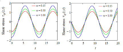
For comparison, Figures 1 and 2 present the time variations of the dimensionless permanent velocities u_{cp}(z,t), u_{sp}(z,t), and shear stresses \tau_{cp}(z,t), \tau_{sp}(z,t), respectively, at the middle of channel for  and three values of the pressure-viscosity coefficient /alpha

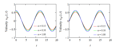
The oscillatory behavior of the two motions and the phase difference between them are clearly visualized. In addition, as expected, the oscillations’ amplitudes of the two motions are identical for same values of physical parameters. Furthermore, as it results from Figures 1, the oscillations’ amplitude is an increasing function with respect to the parameter /alpha It means that fluids with pressure-dependent viscosity flow faster in comparison with ordinary fluids.

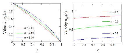
The variations of dimensionless permanent velocity u_{cp} with respect to the spatial variable z and the pressure-viscosity coefficient /alpha are presented in Figures 3. From these figures it clearly results that the fluid velocity is a decreasing function with respect to z and grows up for increasing values of /alpha. Consequently, as before, the fluids with pressure-dependent viscosity flow faster than ordinary fluids and their speed increases as we approach the moving plate. This is possible for pressure-dependent viscosity fluid motions induced by a moving plate because the fluid adheres to the walls and the influence of the plate on the fluid movement brings up increasing fluid viscosity. Boundary conditions are clearly satisfied.

The oscillatory behavior of the fluid motion in the case of the modified second Stokes’ problem confers the essential difference from the modified first Stokes’ problem of the same fluids.

6. Conclusions

As it was previously mentioned, modified Stokes’ problems for a class of incompressible Newtonian fluids with pressure-dependent viscosity are analytically and numerically investigated. The main results that have been brought to light in this short note are:

• Analytic expressions of the dimensionless permanent velocity and shear stress fields corresponding to the modified Stokes’ problems for some fluids with power-law dependence of viscosity on pressure have been provided.
• Similar solutions corresponding to same problems for ordinary incompressible Newtonian fluids have been recovered as limiting cases of general solutions using asymptotic approximations of Bessel functions.
• Graphical representations brought to light some characteristics of the fluid behavior and showed that fluids with pressure-depending viscosity flow faster than ordinary fluids.
• As expected, the fluid velocity increases as we approach the moving plate andthe boundary conditions are clearly satisfied.

Finally, we remember the fact that the steady solutions for unsteady motions of fluids are important in practice to determine the required time to reach the steady state. From mathematical point of view, this is the time after which the diagrams of starting solutions (numerical solutions) superpose over those of steady state solutions. This time is very important for the experimental researchers who want to know the transition moment of the motion to the steady state. In addition, the exact solutions can be also useful to test different numerical schemes that are used to describe more complex fluid motions.

1. M.M. Denn, Polymer Melt Processing, Cambridge University Press, Cambridge, U.K., 2008.
2. K.R. Rajagopal, G. Saccomandi, L. Vergori, “Flow of fluids with pressure and shear-dependent viscosity down an inclined plane,” Journal of Fluid Mechanics, vol. 706, pp. 173–189, 2012, doi:10.1017/jfm.2012.244.
3. G.G. Stokes, “On the theories of the internal friction of fluids in motion, and of the equilibrium and motion of elastic solids,” Transactions of the Cambridge Philosophical Society, vol. 8, pp. 287–305, 1845.
4. P.W. Bridgman, The Physics of High Pressure, MacMillan Company, New York, 1931.
5. E.M. Griest, W. Webb, R.W. Schiessler, “Effect of pressure on viscosity of high hydrocarbons and their mixture,” Journal of Chemical Physics, vol. 29, pp. 711–720, 1958.
6. K.L. Johnson, R. Cameron, “Shear behavior of elastohydrodynamic oil films at high rolling contact pressures,” Proceedings of the Institution of Mechanical Engineers, vol. 182, pp. 307–319, 1967.
7. K.L. Johnson, J.L. Tevaarwerk, “Shear behavior of elastohydrodynamic oil films.” Proceedings of the Royal Society of London, Series A, vol. 356, pp. 215–236, 1977.
8. S. Bair, W.O. Winer, “The high-pressure high shear stress rheology of liquid lubricants,” Journal of Tribology, vol. 114, pp. 1–13, 1992, doi:10.1115/1.2920862.
9. S. Bair, P, Kottke, “Pressure-viscosity relationship for elastohydrodynamic,” Tribology Transactions, vol. 46(3), pp. 289–295, 2003, doi:10.1080/10402000308982628.
10. V. Prusa, S. Srinivasan, K.R. Rajagopal, “Role of pressure dependent viscosity in measurements with falling cylinder viscometer,” International Journal of Non-Linear Mechanics, vol. 47(7), pp. 743–750, 2012, doi:10.1016/j.ijnonlinmec.2012.02.001.
11. K.R. Rajagopal, G. Saccomandi, L. Vergori, “Flow of fluids with pressure and shear-dependent viscosity down an inclined plane,” Journal of Fluid Mechanics, vol. 706, pp. 173–189, 2012, doi: 10.1017/jfm.2012.244.
12. F.J. Martinez-Boza, M.J. Martin-Alfonso, C. Gallegos, M. Fernandez, “High-pressure behavior of intermediate fuel oils,” Energy & Fuels 25(11), pp. 5138–5144, 2011, doi:10.1021/ef200958v.
13. J.M. Dealy, J. Wang, Melt Rheology and Its Applications in the Plastics Industry, 2nd ed., Springer, Dordrecht, The Netherlands, 2013.
14. M. Asif, M. Sajid, M.N. Sadiq, “Investigation of blade coating with pressure-dependent viscosity in couple stress fluid flow,” Journal of Plastic Film & Sheeting 42(1), pp. 51–70, 2025, doi:10.1177/87560879251358512.
15. X. Chen, Z. Xie, Y. Jian, “Streaming potential of viscoelastic fluids with the pressure-dependent viscosity in nanochannel,” Physics of Fluids, vol. 36, Issue 3, 032025, 2024, doi:10.1063/5.0197157.
16. A.Z. Szeri, Fluid Film Lubrication, Cambridge University, Cambridge, 1998.
17. C. Barus, “Note on the dependence of viscosity on pressure and temperature,” Proceedings of the American Academy of Arts and Sciences, vol. 27, pp. 13–18, 1891, doi:10.2307/20020462.
18. C. Barus, “Isothermals, isopiestics and isometrics relative to viscosity,” American Journal of Science, vol. s3-45, Issue 266, pp. 87–96, 1893, doi:10.2475/ajs.s3-45.266.87.
19. K.R. Rajagopal, “Couette flows of fluids with pressure dependent viscosity,” International Journal of Applied Mechanics and Engineering, vol. 9, no.3, pp. 573–585, 2004.
20. F.T. Akyildiz, D. Siginer, “A note on the steady flow of Newtonian fluids with pressure dependent viscosity in a rectangular duct,” International Journal of Engineering Science, vol. 104, pp. 1–4, 2016, doi:10.1016/j.ijengsci.2016.04.004.
21. K.D. Housiadas, G.C. Georgiou, “Analytical solution of the flow of a Newtonian fluid with pressure-dependent viscosity in a rectangular duct,” Applied Mathematics and Computation, vol. 322, pp. 123–128, 2018, doi:10.1016/j.amc.2017.11.029.
22. B. Calusi, L.I. Palade, “Modeling of a fluid with pressure-dependent viscosity in Hele-Shaw flow,” Modelling, vol. 5(4), pp. 1490–1504, 2024, doi:10.3390/modelling5040077.
23. R.S. Herbst, C. Harley, K.R. Rajagopal, “Flow of fluids with pressure-dependent viscosity in intersecting planes,” Fluids, vol. 10(2), 33, 2025, doi:10.3390/fluids10020033.
24. C. Fetecau, Hanifa Hanif, “Long-time solutions of the modified MHD Stokes’ problems for a class of Maxwell fluids with pressure-dependent viscosity. Applications,” Discrete and Continuous Dynamical Systems – Series S, Published online: December 15, 2025, doi: 10.3934/dcdss.2026021.
25. C. Fetecau, “Permanent solutions for MHD modified Stokes’ problems of some Maxwell fluids with power-law dependence of viscosity on pressure,” accepted for publication in journal Annals of Academy Romanian Sciences. Series of Applied Mathematics in 2026.
26. C. Sin, E.S. Baranovskii, Regularity Theory for Generalized Navier-Stokes Equations: Non-Newtonian Fluids with Variable Power-Law, Vol. 10, De Gruyter Series in Applied and Numerical Mathematics, Walter de Gruyter GmbH & Co.KG, 2025.
27. K.R. Rajagopal, G. Saccomandi, L. Vergori, “Unsteady flows of fluids with pressure dependent viscosity,” Journal of Mathematical Analysis and Applications, vol. 404, Issue 2, pp. 362–372, 2013, doi:10.1016/j.jmaa.2013.03.025.
28. D.G. Zill, Free Course in Differential Equations with Modelling Applications, Ninth. ed., BROOKS/COLE, CENGAGE Learning, Australia, United Kingdom, United States, 2009.
29. K.R. Rajagopal, “A note on unsteady unidirectional flows of a non-Newtonian fluid,” International Journal of Non-Linear Mechanics, vol. 17, Issues 5-6, pp. 369–373, 1982, doi:10.1016/0020-7462(82)90006-3.

Citations by Dimensions

Citations by PlumX

Crossref Citations

No related articles were found.