The Taïba Ndiaye wind farm, connected to the SENELEC grid, plays a key role in offsetting shortfalls in electricity consumption, with an installed capacity of 158.7 MW. Moreover, as an intermittent power station, its production is highly dependent on the environmental conditions in the region. Bad weather can disrupt the electricity network, requiring forecasting methods to anticipate its production. This will make it easier to decide how much fossil energy to bring on stream to meet demand. The aim of this paper is to provide forecasts of wind generation at Taïba Ndiaye, subdividing the data into 80% for model training and 20% to assess its robustness to generalization to other situations. The aim is to quantify the energy produced and facilitate an optimal transition between intermittent and fossil energy sources. Two artificial intelligence models classified as machine learning (decision tree and random forest) are proposed in the study, with respective coefficients of determination of 0.92 and 0.938. The results, compared with the literature, demonstrate the reliability of the approach using only production data. These results promise significant benefits in terms of resource management.

1. Introduction 

Prior to the integration of intermittent renewable energies into the power grid, the flow of energy followed a single direction, ensuring greater stability of the power system [1]. Today, however, with the injection of these energies, such as solar and wind power, the energy flow becomes bidirectional, which easily disrupts the grid when faced with rapid variations in meteorological parameters [2]. Furthermore, the injection of these intermittent energies must not exceed 30% of total energy demand in some countries [3]. This presents grid operators with a significant challenge in maintaining a consistent balance between production and consumption to avoid malfunctions, undesirable voltage and frequency variations, and costly imbalances [4]. Network operators must be able to anticipate the production of intermittent power plants in order to adjust the production of fossil fuels, thereby balancing customer consumption with production. Furthermore, in view of global concerns about the fight against climate change, the electricity grids of several countries continue are integrating intermittent energies into their electricity grids, despite the drawbacks [5]. Senegal is following a similar approach, with a 30% increase in the energy mix [6]. These include the Taïba Ndiaye wind farm, with a capacity of 158.7 MW, as well as Malicounda (20 MW), Diass (23 MW), Bokhol (20 MW), etc [7][8]. Against this backdrop of high penetration of intermittent renewable energies, forecasting has become essential to ensure the stability of the electricity network [9]. Several studies have focused on forecasting the potential of renewable resources, whether solar or wind. These studies mainly rely on artificial intelligence models to predict wind energy, given its complex characteristics of continuous production both day and night, which makes this difficult [10]. Indeed, operators face difficulties due to the volatile nature of these sources, with weather parameters requiring constant monitoring to anticipate tasks linked to technical constraints [11]. To overcome these challenges, data science experts are working more closely with grid operators to collect data in order to accurately predict intermittent energy with artificial intelligence (AI) models. AI-based forecasting models are fed by data from sensors installed in the power plant. These models are currently significantly improving the prediction of intermittent power plant output with high accuracy [12][13]. Their reliability in predictive decision-making is no longer in question [14]. In fact, they enable production to be predicted over fairly short time horizons, thus enabling the SENELEC distributor to ensure the stability of network frequency and voltage [8]. Comparative studies have confirmed that these AI models outperform statistical models because of their very satisfactory predictive power [15]. This is evidenced by the studies conducted on the wind power production in Italy and the United States, as well as in Senegal on short-term solar irradiance [16][17]. Despite the robustness and relevance of AI models, their intensive use of data with several input variables to predict the target is not without consequences for computing resources, requiring considerable computing power.  Some experts in the field have highlighted that their machines can sometimes overload, while others have mentioned that the latent time is sometimes too high to obtain optimal results [7]. To address this issue, we propose using two parameter predictors to forecast the short-term power output of the Diass wind power plant, using random forest models and decision trees. These models will be trained using only wind generation measured over a one-year period. The objective is to improve the prediction performance of the wind power plant by reducing the number of input parameters [7]. This paper is structured as follows: the presentation of the data as well as the wind power plant and the method discussed is provided in section II. Section III outlines the AI algorithms used. In Section IV, the results and discussion are presented. Finally, in Section V, the conclusion is provided.

2. Presentation of the plant and data

2.1. Classification of the Taïba Ndiaye wind farm

Wind energy is the kinetic energy generated by the movement of the wind, transformed into mechanical energy by wind turbines and then converted into electrical energy. The energy is given by equation (1). 

$$E = \frac{1}{2} \times A \times \rho \times V^3 \times C_p \times \eta \tag{1}$$

where:

    – 𝐸: is the wind energy produced (in watts or joules),

    – 𝐴: is the area swept by the turbine blades (in square metres),

    – ρ: is the density of the air (in kilograms per cubic metre),

    – 𝑉: is the wind speed (in metres per second),

    – Cp: is the power coefficient of the wind turbine (without unit, a typical maximum value is around 0.59),

    – η: is the mechanical and electrical efficiency of the system (unitless, a typical value is around 0.85).

The value of the power coefficient Cp depends on the speed of rotation of the turbines and the angle of inclination of the blades. Wind turbines are classified into three groups according to propeller diameter and power output [18]. Table I shows a classification of wind turbines:

Table 1: Classification of wind turbines [18]

According to this classification, our study plant, with a capacity of 158.7 MW, is classified as a large wind power plant. It is equipped with the necessary data collection equipment. These enable efficient planning of energy production by anticipating load variations to meet injection requirements. Careful analysis facilitates energy injection, minimizing waste and reducing the costs associated with fluctuations in production. It also facilitates the integration of forecasting models to guarantee operational stability.

2.2. Production data 

Figure 1 illustrates the data obtained from the sensors installed at the wind farm. These data are related to various environmental factors that will be used in our forecasts. The measurements were taken every ten (10) minutes for one year and averaged by hours, days and months. This is a time series with repeating trends at the beginning and end of the year, probably due to favourable weather conditions [8]. Their associated temporal indices are of the order of minutes, hours, days and months. These parameters are crucial for modelling this type of problem. To achieve an accurate prediction, we will incorporate seasonal phenomena, including the temporal indices, into the data reduction process.

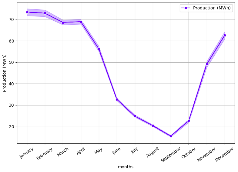
Unlike solar power, wind power generates energy continuously, but this continuity is subject to unpredictable variations due to weather conditions. This intermittent nature of wind generation can sometimes pose complex challenges for electricity network managers. It is therefore important to keep a close eye on environmental parameters such as wind speed and direction, as they are closely linked to wind power generation. These variations can be rapid and significant, requiring proactive management to ensure grid stability. By understanding and anticipating these intermittencies, managers can take appropriate measures to maintain a reliable electricity supply.

2.3. Wind speed data  

The power law also known as Murphy’s law is a widely used approach to modelling wind speed [19],[20]. It states that the wind speed V at a given height above the ground is proportional to the power of the height h. Its mathematical relationship is given by equation (2) [19]:

$$V = V_{\text{ref}} \left( \frac{h}{h_{\text{ref}}} \right)^{\alpha} \tag{2}$$

where:
– V: is the wind speed at height h,
– 𝑉ref: is the wind speed at a reference height ℎref,
– α: is the exponent of the power law, which depends on  local site conditions and terrain characteristics.

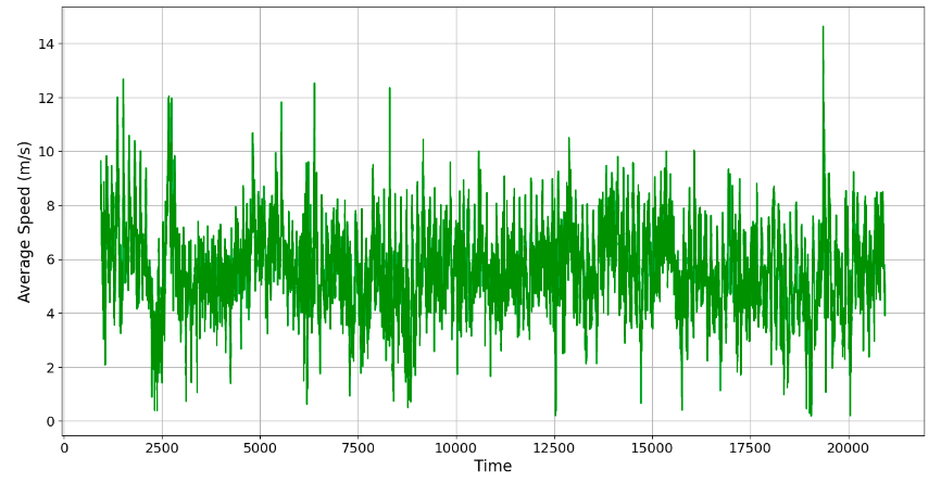
From the modelling, the wind speed can be collected at the wind turbine installation site. The variation in mean wind speed at the Taïba Ndiaye site is shown in Figure 2.

It shows the typical fluctuations in wind speed, which are characterised by periods of rise and fall. These fluctuations are often influenced by specific weather conditions and are continuous throughout the day, month and year. This continuous variation in wind speed presents a significant challenge when predicting wind generation. It is particularly complex because of this variability. Indeed, this variability in wind speed can lead to rapid changes in energy production, requiring dynamic management of energy resources to maintain the stability of the power grid. This requires the use of advanced modelling and simulation techniques, as well as artificial intelligence algorithms capable of analysing large datasets and recognizing complex patterns.

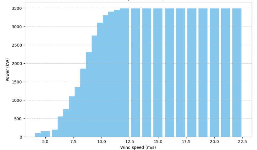
Given the wind speed data, a wind turbine with the power curve shown in Figure 3 was chosen for the model.

The turbine’s power increases until it reaches a speed of 12 m/s, where it remains constant until 22 m/s, which could correspond to the turbine’s stall speed. This indicates that the turbine is designed to operate optimally within a predefined range of wind speeds. The turbine reaches its maximum rated output at a wind speed of 12 m/s. During this period, the turbine makes full use of the available kinetic energy of the wind. The turbine’s power remains constant above the rated speed, up to 22 m/s. This mechanism is designed with an effective control system to prevent overloads and damage caused by excessively high wind speeds. In fact, the stall system protects the wind turbine and guarantees the durability of the components while stabilising the electricity. For accurate prediction purposes, it is important to take these wind fluctuations into account to provide a model capable of accurately predicting wind energy production. However, wind direction is one of the elements that creates turbulence, which is synonymous with wind fluctuations. It can have a positive influence on wind installations and their production.

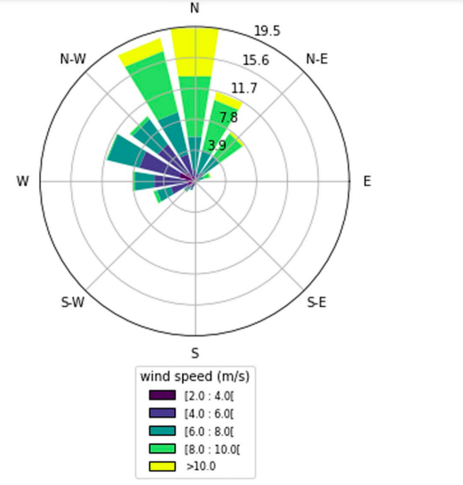
2.4. Wind direction data

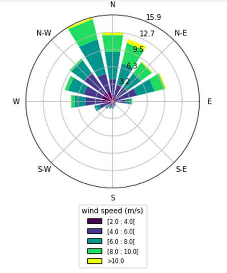
The wind direction mainly shows that the winds blow in the optimum directions. These predominant wind directions correspond to the periods of maximum production for the wind power plant. Figures 4 and 5 show the predominant wind directions during the day and night respectively in the Taïba Ndiaye area. Figure 4 shows that the predominant wind direction from south-east to north-west during the day, it can be seen that the highest wind speeds are between 6 m/s and 8 m/s. Wind speeds of up to 10 m/s are fairly limited. At night, on the other hand, the prevailing winds blow from south to north at speeds of around 10 m/s. This observation shows that the wind farm’s output is higher at night. It is therefore important to carefully monitor of these wind data in order to guarantee optimum energy feed-in to the power grid. By monitoring and anticipating variations in wind direction and speed, operators can adjust the plant’s output accordingly. This not only optimises the production of wind energy, but also its smooth integration into the electricity grid, contributing to a more stable and reliable power supply for consumers.

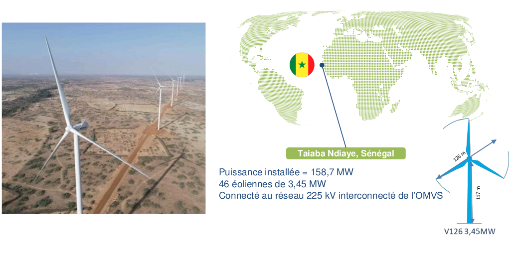
2.5. Presentation of the plant

At Taïba Ndiaye, the data collected come from the wind power plant, which is an impressive installation consisting of 46 Vesta V 126-3.45 wind turbines. The plant is equipped with a collector that feeds two 33/225 kV, 80/100 MVA step-up transformers, which gives it significant generating capacity [21]. The plant is strategically connected to the interconnected 225 kV network of the Organisation pour la Mise en Valeur du Fleuve Sénégal (OMVS), with an installed capacity of 158.7 MW. Figure 6 provides a clear illustration the installed wind farm and its characteristics. It is located in an open area and is well positioned to capture the wind. The meteorological data showed the dominant wind directions, as illustrated in Figures 4 and 5. It is important for the production of renewable energy and contributes significantly to the energy mix in the electricity grid.  

The importance of this data goes beyond simply monitoring solar production. By analysing this data, researchers may be able to gain a deeper understanding of the plant’s current performance, as well as develop predictive models to anticipate seasonal and meteorological variations.

3. Prediction Algorithms

In this section, the two used prediction algorithm (the decision tree and the random forest algorithm) are presented.

3.1. Decision Tree Model

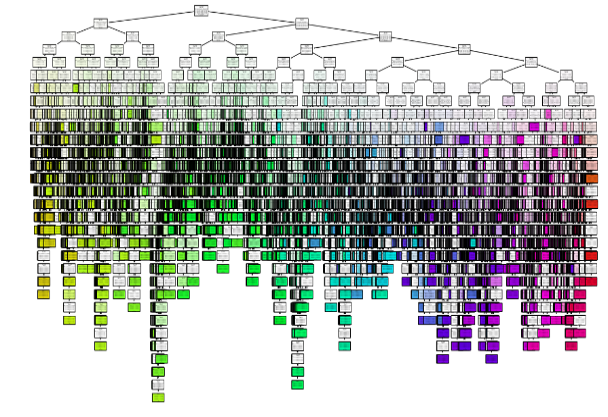
The decision tree is a classification and regression tree.  The configuration of the tree is shown in Figure 7 and consists of the following elements:

    – Root node: This represents the highest points in the figure 7.

    – Internal nodes: These correspond to tests formulated in the form of questions on the characteristics of the parameters in relation to the target to be predicted.

    – Branches: These present the results of the tests, and according to these answers, the subdivision is made as observed in figure 7.

    – Leaf nodes: These nodes represent a decision.

The partition equation of each node into two classes is given by (3)[14]:

$$X : X_j \leq s = C1(j,s) \quad X : X_j > s = C2(j,s) \tag{3}$$

The couple (j, s) designate the partition limit of the data that we try to predict. Here, the goal is to find the boxes      C1, …, CJ that minimize the least squares criterion, represented by (4) according to [22]:

$$\sum_{j=1}^{k} \sum_{i \in R_j}^{N} (Y_i – \hat{Y}_j)^2 = \text{SSE} \tag{4}$$

Where Y_i and Ŷ_t refers to the actual and the predicted values respectively and SSE Residual Sum of Squares.

The forecasting task involves explaining the target variable Y (plant output) as a function of a set of explanatory variables X (measurement times, day number and month). Thus, the different modalities of the X explanatory variables are examined using the chi-square test to determine which variables are closely related to the Y target. When the p-value of the chi-square test is less than 0.05, we conclude that the variable is significantly associated with the target variable Y. This criterion is particularly important when the learning loop is interrupted, ensuring that all nodes have chi-square tests greater than 0.05, indicating the absence of a strong association between the explanatory variables X and the target variable Y.

3.2. Random Forest Model

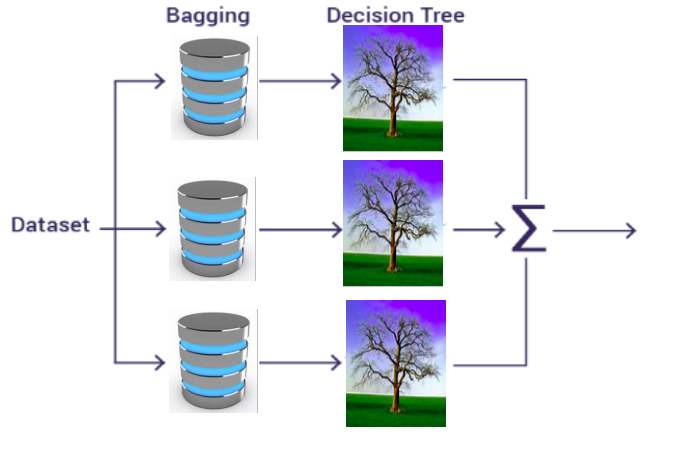
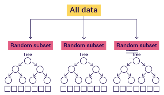
This model consists of a collection of several decision trees trained using the Bagging method. The algorithm is applied in three stages:
-Bagging: this is a technique that involves grouping several decision trees together to obtain a final result, rather than relying on individual decision trees. Figure 8 shows its format

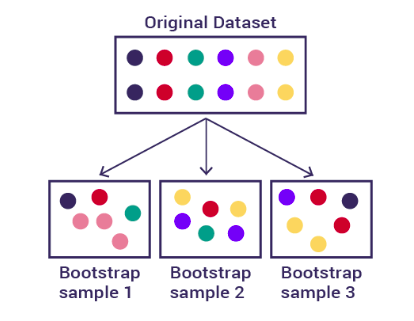
-Bootstrapping: This is a process that begins with the application of the bootstrap technique, which is a sampling method as shown in Figure 9. This approach involves creating random subsets from the initial dataset, using N samples. The N samples are selected with replacement, allowing the same sample to be included several times in the subset.

-Bagging aggregation: In the bagging aggregation phase, each random subset is subjected to a decision tree algorithm. The final result is obtained by taking the average of all the predictions generated by the different trees, as shown in Figure 10.

3.3. Performance Evaluation Criteria

The evaluation of the performance of our forecasts is based on the criteria defined by equations (5), (6), (7) and (8), where N represents the total number of values contained in the data [16], [23]. These indices provide a basis for judging comparisons with a view to future model improvements. However, comparison between models remains complex due to differences in forecast horizons, number of input parameters and meteorological conditions. Nevertheless, the mean absolute error (MAE), as defined in equation (5), is particularly relevant for linear cost functions, providing a proportional measure of prediction errors. In contrast, the root-mean-square error (RMSE) (6) is more suitable for significant deviations between forecast and observation. On the other hand, the root mean square error (RMSE), as defined in equation (7), is very responsive to these deviations, making it a valuable comparative parameter, particularly suitable for public applications [23]. It is worth noting that the lower the RMSE or MAE, the better the quality of the production forecast for our wind farm.

$$\frac{1}{N} \sum_{i=1}^{N} |Y_i – \hat{Y}_t| = \text{MAE} \tag{5}$$

$$\sqrt{ \frac{1}{N} \sum_{i=1}^{N} (Y_i – \hat{Y}_t)^2 } = \text{RMSE} \tag{6}$$

$$\frac{1}{N} \sum_{i=1}^{N} (Y_i – \hat{Y}_t)^2 = \text{MSE} \tag{7}$$

$$1 – \frac{ \sum_{i=1}^{N} (Y_i – \hat{Y}_t)^2 }{ \sum_{i=1}^{N} Y_i^2 } = R^2 \tag{8}$$

All these equations evaluate the parameters used to measure the accuracy of the power predicted by the algorithms of the two models used.

3.4. Flowchart of the Artificial Intelligence Model Algorithm

The flowchart of the regression tree and forest type artificial intelligence algorithm is a representation of the sequences and decisions to be taken by the algorithm to predict numerical values of the wind production of the targeted Taïba Ndiaye. In this work, it is described as follows:

Begin  

1. Enter the historical wind production data for Taïba Ndiaye.
2. Convert all data to hourly resolution by averaging.
3. Select the target variable to be predicted (energy produced per hour).
4. Apply WT decomposition (hierarchical multi-step decomposition) to historical target data (wind power).
5. Identify training (80%) and test (20%) data sets.
6. Verify tree convergence during model training.
7. Save the trees if the convergence condition is met (these saved trees are called Wind Production Forecasters).
8. If not, move on to the application of model hyper-parameters.
9. Recheck the convergence of the trees during training.
10. Save the trained shafts if the convergence condition is met.

4. Results and Discussion

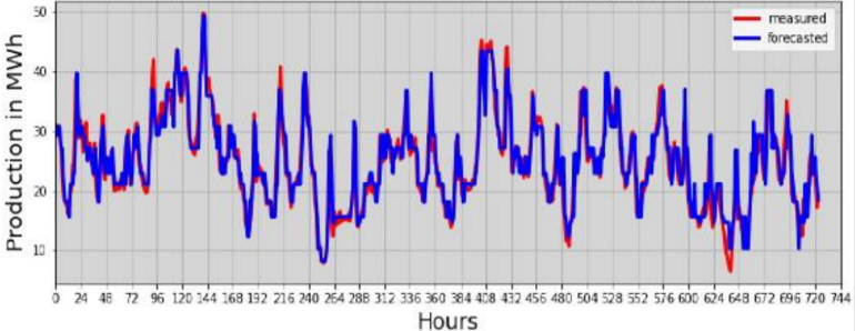
TShort-term forecasting is of paramount importance in managing the distribution of wind generation throughout the year. It also offers managers the possibility of making real-time adjustments within the electricity network integrating intermittent renewable energies [24]. However, we have chosen to focus on the months of January and July, as they respectively encompass the most significant and least significant production of the year. The data was collected during this period. In fact, if the models manage to make a good prediction, then its generalisation to the other months of the year is quite obvious. Figures 11 and 12 illustrate the predictions generated by the two AI models for the month of January, when production rose. These graphical representations compare actual wind energy production with the one-hour forecasts. Indeed, a relevant method for evaluating the performance of a forecast consists of anticipating previously observed data based on the data that preceded it. By analysing these predictions for the month of January with the highest production provides an in-depth view of the models’ ability to accurately anticipate variations in the wind power plant.

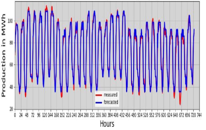
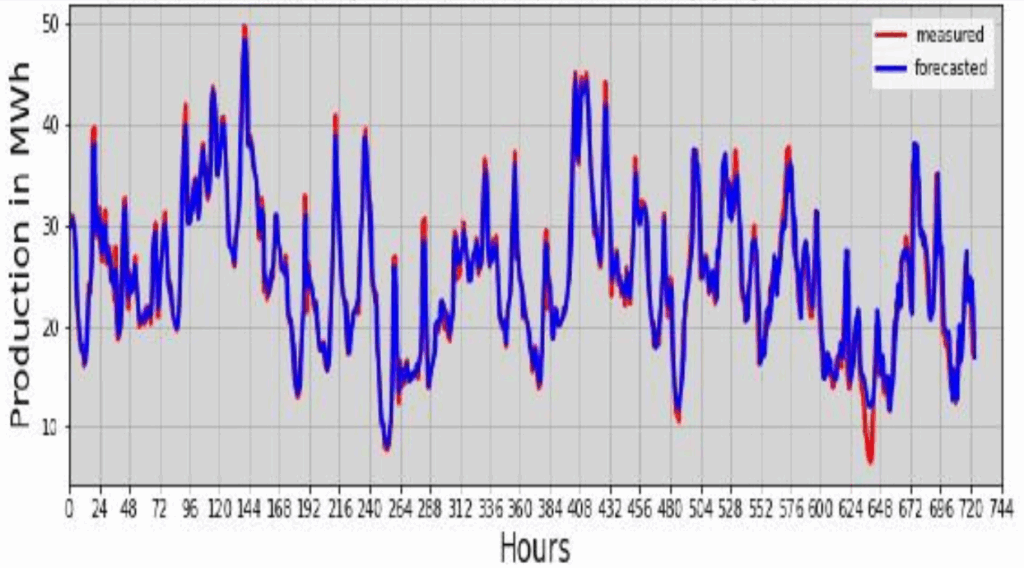
The graphs above appear to show a potential correlation between the predictions (in blue) and the plant’s actual output (in red) for the month of January, with RMSEs of 0.527 and 0.3332 Mwh/day respectively for the decision tree and random forest models. At the start of production, observations suggest that there may be occasional discrepancies between prediction and reality. These discrepancies are sometimes manifested by a much higher predicted production or, conversely, by an actual production at the lower limit of the prediction, for both models. It should be noted, for example, that except for day 27 (648 hours on the curve, Fig. 12), the observed values exceed the prediction of the random forest model from day 21 (504 minutes on the curve) to day 28 (672 hours on the curve), generally around 11pm. Despite a lower RMSE for the random forest model, these days show a better match between the predictions of the decision tree model and the actual observations (see Fig. 11). This observation reveals some interesting nuances in the evaluation of performance with respect to the two models. This suggests that the RMSE metric alone may not fully capture the reliability of the models in specific situations. On the other hand, these differences do not appear uniformly for all the days of the month for which production is predicted. A general trend emerges, indicating that in most cases the random forest model provides more accurate forecasts than the decision tree model. It seems that the latter may be more effective in forecasting resources during low production hours. This could be attributed to the optimisation criterion favouring the homogeneity of the descendants with respect to the target variable. In other words, the variable tested in the node will be the one that maximises this homogeneity.

Furthermore, a particularly useful complementarity effect emerges in both models. During periods of increased production, the prediction of the random forest model stands out for its greater accuracy. The algorithm underlying the random forest performs its training on several trees formed from various subsets of data, thus conferring a complementarity that reinforces the effectiveness of the current hybrid models with better prediction. The coefficients of determination between the actual values and those predicted by the models reached 0.92 and 0.9382 respectively for the decision tree and the random forest during the month of January. 

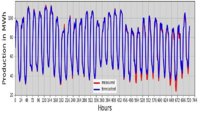
Fig 13 and 14 show a comparison between the values observed and predicted by the two models for the month of July. This is the month of the year when the plant supplies less energy to SENELEC. We also note that the predictions closely follow the actual production curve, with few systematic errors or apparent peaks (see Fig. 13 and Fig. 14). This consistency underlines the robustness of the models in predicting wind generation, irrespective of significant seasonal variations.

On the 26th day (624 hours of the curve) at around 11pm, a peak was observed for both models, although it did not affect the forecasts for the following hours.

The coefficients of determination were 0.76 for the decision tree and 0.794 for the random forest. These values are lower than those observed in January. When production falls, these coefficients show little variability, often attributable to unforeseen adverse weather conditions impacting production. It can sometimes be challenging to predict this with certainty.

A comprehensive examination of the error behaviour of each model over the month of July reveals slight differences (1.74 Mwh/m2/day for the tree model (see Fig.13) and 1.027 Mwh/m2/day (see Fig.14). These discrepancies can be attributed to the random nature of the seasonal variation in the study area and by the potential issue of underlearning.

The performance criteria, evaluated by the models [17] [25], [26] are used to examine the impact of the parameters and are applied to the test data to generalise the artificial intelligence models. In the study, a slight decrease in performance was observed for the different days of the predicted months. The summary of the performance parameters studied for the months of January and July are presented in Table II. The performance indices obtained are compared with those reported in the state of the art, with the aim of highlighting the limited number of input parameters used during model training. Despite this limitation, the learning techniques succeed in reducing the error, which illustrates the performance obtained. This performance is made possible in part by variations in tree depth.

Table 2: Comparison of performance indices

5. Conclusion

The strategy of increasing the share of renewable energies in the energy mix, while important for achieving sustainable development objectives, presents significant operational challenges. Indeed, this expansion leads to imbalances in the electricity network, causing excessive maintenance costs. Considering these challenges, it is becoming increasingly clear that accurate prediction of energy production is essential to guide decisions while anticipating operational requirements.

In order to achieve this goal, this article presents two artificial intelligence models, based on the decision tree and the random forest, with the intention of increasing the accuracy of forecasts for the Taïba Ndiaye power plant. The models were trained on the plant’s production parameters over a one-year period. The results obtained demonstrate that, even in the absence of direct integration of meteorological parameters into the models, the proposed method allows for the robust prediction of wind power over a one-hour horizon. The coefficients of determination R2 were 0.92 and 0.938 respectively for the decision tree and random forest models. The root mean square error (RMSE) values of 0.3332 MWh and 0.527 MWh for the random forest model and decision tree respectively, reflect the considerable potential of AI models commonly referred to as machine learning in wind power forecasting. Overall, these results offer a promising prospect for optimising the penetration rate of intermittent energies such as wind power in the electricity grid. Nevertheless, we intend to utilise neural networks to enhance the plant’s forecasts with the objective of further optimising the quality of the energy injected into the SENELEC electricity network.

Conflict of Interest

The authors declare no conflict of interest.                                                                                              

1. W. Zappa, M. Junginger, and M. van den Broek, “Is a 100% renewable European power system feasible by 2050?” Applied Energy, vol. 233–234, pp. 1027–1050, 2019.
2. A. Jamil, M. Imran, S. H. Ahmed, and A. Anpalagan, “Challenges and opportunities in wind power integration,” IEEE Access, vol. 6, pp. 63211-63233, 2018.
3. A. Fischer, L. Montuelle, M. Mougeot, and D. Picard, “Statistical learning for wind power: A modeling and stability study towards forecasting,” Wind Energy, vol. 20, no. 12, pp. 2037-2047, 2017.
4. M. Dieng, A. Ndoye, M. S. Sow, and A. Wane, “Energy consumption forecasting using artificial neural networks: A case study of Senegal,” 2015 IEEE International Conference on Industrial Technology (ICIT), Seville, Spain, 2015, pp. 2432-2437.
5. K. Jha, & A. G. Shaik, “A comprehensive review of power quality mitigation in the scenario of solar PV integration into utility grid,” E-Prime – Advances in Electrical Engineering, Electronics and Energy, vol. 3, 100103, 2023. https://doi.org/10.1016/j.prime.2022.100103.
6. A.S. Ba, (2018). “The energy policy of the Republic of Senegal.”.
7. S. Diop, P. S. Traore, & M. L. Ndiaye, “Power and Solar Energy Predictions Based on Neural Networks and Principal Component Analysis with Meteorological Parameters of Two Different Cities: Case of Diass and Taïba Ndiaye,” 2022 IEEE International Conference on Electrical Sciences and Technologies in Maghreb (CISTEM), vol. 4, pp. 1-6, IEEE, October 2022.
8. S. Diop, P. S. Traore, and M. L. Ndiaye, “Wind Power Forecasting Using Machine Learning Algorithms,” 2021 9th International Renewable and Sustainable Energy Conference (IRSEC), 2021, pp. 1-6, doi: 10.1109/IRSEC53969.2021.9741109.
9. M. Shafiullah, S. D. Ahmed, & F. A. Al-Sulaiman, “Grid Integration Challenges and Solution Strategies for Solar PV Systems: A Review,” IEEE Access, vol. 10, pp. 52233–52257, 2022. https://doi.org/10.1109/ACCESS.2022.3174555.
10. A. Kaur, L. Nonnenmacher, and C. F. M. Coimbra, “Net load forecasting for a hybrid renewable energy system based on receding horizon optimization,” Energy, vol. 150, pp. 617-630, May 2018.
11. J. Maldonado-Correa, M. Valdiviezo, J. Solano, M. Rojas, and C. Samaniego-Ojeda, “Wind energy forecasting with artificial intelligence techniques: A review,” International Conference on Applied Technologies, December 2019, pp. 348-362. Springer, Cham.
12. S. Noman, A. A. Roya, K. Lauri, N. I. Muhammad, and R. Argo, “Forecasting Short Term Wind Energy Generation using Machine Learning,” Conference Paper, October 2019, PSG 142. DOI: 10.1109/RTUCON48111.2019.8982365.
13. T. Mahmoud, Z. Y. Dong, and J. Ma, “An advanced approach for optimal wind power generation prediction intervals by using self adaptive evolutionary extreme learning machine,” Renewable Energy, vol. 126, pp. 254–269, 2018.
14. G. Notton, M. L. Nivet, C. Voyant, C. Paoli, C. Darras, F. Motte, and A. Fouilloy, “Intermittent and stochastic character of renewable energy sources: Consequences, cost of intermittence and benefit of forecasting,” Renewable and Sustainable Energy Reviews, vol. 87, pp. 96-105, 2018.
15. Y.-J. Ma, & M.-Y. Zhai, “A Dual-Step Integrated Machine Learning Model for 24h-Ahead Wind Energy Generation Prediction Based on Actual Measurement Data and Environmental Factors,” Applied Sciences, vol. 9, no. 10, 2125, 2019. doi:10.3390/app9102125.
16. W. M. Nkounga, M. F. Ndiaye, M. L. Ndiaye, O. Cisse, M. Bop, & A. Sioutas, “Short-term forecasting for solar irradiation based on the multi-layer neural network with the Levenberg-Marquardt algorithm and meteorological data: application to the Gandon site in Senegal,” 2018 7th International Conference on Renewable Energy Research and Applications (ICRERA), 2018. doi:10.1109/icrera.2018.8566850.
17. A. Clifton, L. Kilcher, J. K. Lundquist, & P. Fleming, “Using machine learning to predict wind turbine power output,” Environmental Research Letters, vol. 8, no. 2, 024009, 2013.
    doi:10.1088/1748-9326/8/2/024009.
18. M. F. Ndiaye, “Supervision de système multi-sources d’énergie,” Thèse Doctoral, Université Cheikh Anta Diop de Dakar- École Supérieure Polytechnique, 2019.
19. F. Pelletier, “Conception d’un site d’évaluation des performances d’éoliennes hors réseau en milieu complexe,” Doctoral dissertation, École de technologie supérieure, 2003.
20. R. Baïle, “Analyse et modélisation multifractales de vitesses de vent. Application à la prévision de la ressource éolienne,” Doctoral dissertation, Université Pascal Paoli, 2010.
21. S.A.A. Niang, M.S. Drame, A. Gueye, A. Sarr, M.D. Toure, D. Diop, S.O. Ndiaye, & K. Talla, “Temporal dynamics of energy production at the Taïba Ndiaye wind farm in Senegal,” Discov Energy, vol. 3, art. 6, 2023. https://doi.org/10.1007/s43937-023- 00018-0.
22. T. R. Prajwala, “A Comparative Study on Decision Tree and Random Forest Using R Tool,” International Journal of Advanced Research in Computer and Communication Engineering, vol. 4, no. 1, January 2015.
23. C. Voyant, G. Notton, S. Kalogirou, M. L. Nivet, C. Paoli, F. Motte, and A. Fouilloy, “Machine learning methods for solar radiation forecasting: A review,” Renewable Energy, vol. 105, pp. 569–582, 2017. doi: 10.1016/j.renene.2016.12.095.
24. H. M. Diagne, M. David, P. Lauret, J. Boland, and N. Schmutz, “Review of solar irradiance forecasting methods and a proposition for small-scale insular grids,” Renewable and Sustainable Energy Reviews, vol. 27, pp. 65-76, 2013.
25. T. Brahimi, “Using Artificial Intelligence to Predict Wind Speed for Energy Application in Saudi Arabia,” Energies, vol. 12, no. 24, 4669, 2019. doi:10.3390/en12244669.
26. E. F. Alsina, M. Bortolini, M. Gamberi, and A. Regattieri, “Artificial neural network optimization for monthly average daily global solar radiation prediction,” Energy Conversion and Management, vol. 120, pp. 320–329, July 2016.

Citations by Dimensions

Citations by PlumX

Crossref Citations

This paper is currently not cited.

No. of Downloads per Month

No. of Downloads per Country