Keratoconus Disease Prediction by Utilizing Feature-Based Recurrent Neural Network

(This article belongs to the Section Biomedical Engineering (BIE))
Export Citations
Cite
Musa, S. H. , Alhaidar, Q. J. M. and Elmi, M. M. B. (2024). Keratoconus Disease Prediction by Utilizing Feature-Based Recurrent Neural Network. Journal of Engineering Research and Sciences, 3(7), 44–52. https://doi.org/10.55708/js0307004
Saja Hassan Musa, Qaderiya Jaafar Mohammed Alhaidar and Mohammad Mahdi Borhan Elmi. "Keratoconus Disease Prediction by Utilizing Feature-Based Recurrent Neural Network." Journal of Engineering Research and Sciences 3, no. 7 (July 2024): 44–52. https://doi.org/10.55708/js0307004
S.H. Musa, Q.J.M. Alhaidar and M.M.B. Elmi, "Keratoconus Disease Prediction by Utilizing Feature-Based Recurrent Neural Network," Journal of Engineering Research and Sciences, vol. 3, no. 7, pp. 44–52, Jul. 2024, doi: 10.55708/js0307004.
Keratoconus is a noninflammatory disorder marked by gradual corneal thinning, distortion, and scarring. Vision is significantly distorted in advanced case, so an accurate diagnosis in early stages has a great importance and avoid complications after the refractive surgery. In this project, a novel approach for detecting Keratoconus from clinical images was presented. In this regard, 900 images of Cornea were used and seven morphological features consist of area, majoraxislength, minoraxislength, convexarea, perimeter, eccentricity and extent are defined. For reducing the high dimensionality datasets without deteriorate the information significantly, principal component analysis (PCA) as a powerful tool was used and the contribution of different PCs are determined. In this regard, Box plot, Covariance matrix, Pair plot, Scree Plot and Pareto plot were used for realizing the relation between different features. Improved recurrent neural network (RNN) with Grey Wolf optimization method was used for classification. Based on the obtained results, the average prediction error of the visual characteristics of a patient with keratoconus six and twelve months after the Kraring ring implantation using RNN are 9.82% and 9.29%, respectively. The average error of estimating characteristics of predicting the visual characteristics of a patient with keratoconus six and twelve months after myoring ring implantation are 11.46% and 7.47% respectively.
1. Introduction
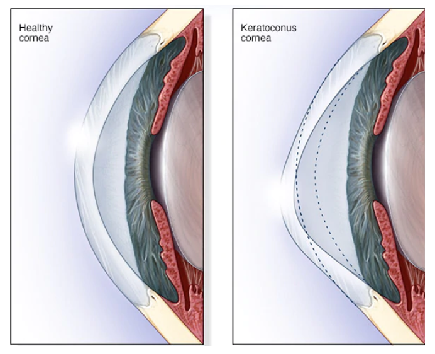
The cornea is the outer layer of the eye, so the structural and repair properties of the cornea are essential for protecting the inner contents, maintaining the shape of the eye and achieving light refraction. Keratoconus is a noninflammatory disorder marked by gradual corneal thinning, distortion, scarring, along with increasing corneal high-order aberrations [1]. Keratoconus’ pathogenic mechanisms have been studied for a very long time. The course of the disease is evidenced by a loss of visual acuity that cannot be compensated by using glasses. Corneal thinning commonly precedes ectasia and diagnosing keratoconus is part of the preoperative examination of patients undergoing corneal refractive surgery (LASIK, PRK, SMILE) and some intraocular surgery patients who desire optimal refractive outcomes (such as premium intraocular lenses for cataract surgery, secondary phakic intraocular lenses, etc) [2]. The function
of the cornea is to clarify the front surface of the eye, which the keratoconus disease changes it into a cone shape (Figure 1). Traditionally, corneal topography, which measures the anterior curvature of the eye, was used to detect Keratoconus. In the early stages of keratoconus and without clinical signs, diagnosis of disease is difficult [3].
In recent years, corneal biomechanics (the corneal response to stress and the cornea’s ability to resist deformation/distortion) is being used to diagnose patients with corneal ecstatic disorders (such as keratoconus) because these conditions are characterized by inherent weaknesses in the cornea’s biomechanical properties. Keratoconus (KTC) is detected in 1 out of every 2000 people in general [4].
In keratoconus, corneal pressure is no longer maintained by the cornea due to structural abnormalities produced by corneal thinning. Consequently, the cornea deforms into a conical shape. Vision is significantly distorted in advanced case, so an accurate diagnosis in early stages has a great importance and avoid complications after the refractive surgery. In the advanced stages of this disease, the cornea completely changes shape and the patient needs a cornea transplant.
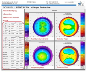
Thanks to the technical advances in image processing, it is possible to diagnose this disease in a reliable and non-invasive way. Typically keratoconus specialists using manual assessment to evaluate different corneal attributes and sometimes embrace machine learning techniques to predict the presence of disease [6]. In other side, corneal topography is prepared by devices such as Pentacam and Erbscan. The Pentacam device is one of the most advanced corneal imaging devices, which not only provides very accurate images of the cornea in a very short time, but also enables the examination and analysis of the characteristics of other interior parts. Usually, on the first page of the pentacam report, four cornea maps are placed next to each other (Figure 2). These four maps are:
- Corneal curvature map
- Height map of the anterior surface of the cornea
- Height map of the posterior surface of the cornea
- Corneal thickness map [7].
In [8], the authors extracted features using four Pentacam-generated refractive maps and retrieved 12 features from each map based on particular diameters. They built a dataset consisting of 40 patients in total and used 30 patients for training and 10 for testing, then obtained results with 90% accuracy. In [9], support vector machine classifier was used, 22 features were extracted from Pentacam and their dataset consisted of 860 patients. They used 10-fold cross validation to train and validate their models and obtained cross-validation accuracies of 98.9%, 93.1% and 88.8% for three different classifiers.
In [10], a 2-way classifier for distinguishing between early stage Keratoconus and normal eyes was presented. The writers compared 25 machine learning models and achieved a test accuracy of 94% using 8 features and a dataset of 3151 patients. Writers of [11] proposed a deep learning approach to classify between Keratoconus and normal eyes. They used data from 304 Keratoconus and 239 normal eyes and reported an accuracy of 0.991 in classifying. In [12], an innovative neural network structure is used. In the designed approach, image and clinical risk factor data are applied as an input data to the multilayer perceptron layer to estimate the disease and in order to improve the results, reinforcement learning techniques have also been evaluated. With considering the potential of severe surgical infections, special precautions must be observed [13].
In Table. 1 the review of comparison between different method are shown. From the review of the articles, it can be achieved that the combination of recurrent neural network with feature extraction classification methods has not been used to identify the disease through medical image processing. The proposed approach not only has proper accuracy, but it is also able to be used well for patients who have passed a long time since their kaeraring and myoring operations and has high flexibility in identifying the disease in various conditions. The main contributions of this paper are as follows:
- Combine the recurrent neural network with PCA-based feature selection methods for improving the efficiency of disease identification.
- Applying different classification methods such as logistic regression (IR), k-nearest neighbors (KNN) and decision tree (DT) on dataset and comparing the results.
- Using many criterias such as Confusion Matrix, Decision Boundary, Prediction error and F-1 score for extracting the main features of images.
- Evaluating the presented approach on data set which is gathered after keraring and myoring operations.
Table 1: Comparison between different results of literatures
Ref. | Dataset (images) | Approach | Accuracy |
[9] | 3510 | SVM | > 98% |
[11] | 546 | CNN | > 99% |
[12] | 570 | MLP | > 83% |
[14] | 2140 | AlN | > 92% |
[15] | 3395 | CNN | > 78% |
[16] | 857 | FNN | > 96% |
[17] | 510 | RF | > 75% |
In order to explain the proposed approach and present the obtained results, the structure of this article continues as follows. In the next part, feature selection methodology and it’s importance for classification algorithms is discussed. Then the steps of applying principal component analysis method on extracted data are presented. After that, characteristics of recurrent neural network are described. In the fifth section, objective function as well as useful benchmarks in this project are formulated. Then, components of data set are defined. Next simulation results after applying PCA and Shapley analysis methods are presented. In this section, four different scenarios for keratoconus classifications after keraring and myoring operations are defined and their results are compared to each other. Before the conclusion section, comparison between different approaches are done for analyzing the efficiency of proposed approach.
2. Basic Concepts
2.1. Feature Selection
Feature selection method is a powerful tool in machine learning and has a great role in clinical intelligence operations. Having a lots of processing capacity and spending a long time to work on the data sometimes is not enough to extract useful information, so it is necessary to use appropriate alternatives to operate with this dataset. There are four important reasons why feature selection is essential:
- Spare the model to reduce the number of parameters.
- Decrease the learning time.
- Reduce overfilling by improving the generalization.
- Avoid the problems of dimensionality [18].
One of the effective solutions to improve the processing efficiency with considering the quality of the results at the proper level, is using principal component analysis (PCA). PCA help to reduce the size of the huge dataset while considering the original features. In this method, by removing many of the obtained features, the average accuracy of the results can be kept more than 70%.
2.2. Principal component analysis
Suppose there is a data set in the form of a matrix with dimensions . In order to implement the PCA method, four steps are defined:
2.2.1. Standardization
In order to normalize, average value for each column is calculated according to (1). Then the central matrix is obtained according to the (2).
$$\bar{x} = \frac{1}{n} \sum_{i=1}^{n} x_i \tag{1}$$
$$\ Y = H \cdot X \tag{2}$$
Here: 𝑥̅ – is a mean vector;
𝑌 – is a centered data matrix;
𝑋 – is a centring matrix.
2.2.2. Covariance matrix computation
Sometimes, the variables are very close to each other, so in these situations, by removing similar ones, it is possible to improve the processing efficiency without causing a significant decreasing in the accuracy. This matrix is calculated as (3) and S is a covariance matrix.
$$S = \frac{1}{n – 1} Y^T Y \tag{3}$$
Here: 𝑆 – is a covariance matrix.
2.2.3. Eigen decomposition
In this step, the eigenvalues and eigenvectors of S are calculated. The obtained results show the direction and variation of each principal components (PCs) (Equation (4)). In this equation, 𝐴 is a orthogonal matrix of eigenvectors and Λ represents diagonal matrix of eigenvalues.
$$S = A \cdot \Lambda \cdot A^T \tag{4}$$
where: 𝐴 – is a orthogonal matrix of eigenvectors;
Λ – is a diagonal matrix of eigenvalues.
2.2.4. Principal Components
In the last step, transfer matrix (z) is calculated which rows represent observations and columns represent PCs (Equation (5)).
$$Z = Y \cdot A \tag{5}$$
2.3. Recurrent Neural Network
The artificial neural network (ANN) technique is a computer-based approach that does not require an estimator to model the system under study [19]. In this method, the patterns are constructed from previous system data and then a mapping is created between the input variables and desired outputs, which is then estimated in order to perform the estimation. In the last decade, neural networks have been made up of multiple layers, known as recurrent neural networks (RNNs). RNNs are a family of algorithms that can include dependency factors between successive time steps. However, as demonstrated by writers of [20], the proposed approach suffers from a gradient divergence pattern that can make factor participation difficult in the long run.
It must be noted that the use of long short-term memory units (LSTM) could be a solution to overcome the problem of gradient divergence. In other side, A RNN is a type of ANN that simulates discrete-time dynamic systems. The structure of such a network is expressed by (6) and (7) [21]. Having a set of N sequences of training data (Equation (8)), RNN parameters are estimated by minimizing the cost function (Equation (9)). RNN parameters should be calculated by a technique such as stochastic gradient descending (SGD) algorithm and by taking the gradient from the cost function expressed in (10) [22]. In the standard RNN structure, the range of accessible content is very limited in practice.
$$h_t = f_h(x_t, h_{t-1}) \tag{6}$$
$$y_t = f_o(h_t) \tag{7}$$
$$D = \left\{ (x_1^{(n)}, y_1^{(n)}), \ldots, (x_{T_n}^{(n)}, y_{T_n}^{(n)}) \right\}_{n=1}^N \tag{8}$$
$$J(\theta) = \frac{1}{N} \sum_{n=1}^N \sum_{t=1}^{T_n} d\left(y_t^{(n)}, f_o(h_t^{(n)})\right) \tag{9}$$
$$h_t^{(n)} = f_h(x_t^{(n)}, h_{t-1}^{(n)}) \tag{10}$$
Here: 𝑡 – is time;
𝑥𝑡– is input;
ℎ𝑡 – is hidden state;
𝑦𝑡– is output;
𝑓ℎ– is state transition function;
𝑓𝑜 – is output function.
The problem is that the influence of a given input on the hidden layer and thus on the entire network decays exponentially and vanishes. This problem is known as gradient fading. In 1977, the long short-term memory (LSTM) neural network was introduced by Hackertier and Schmidber, in which the neurons of the hidden layer were replaced by memory blocks, and thus the challenge of long sequences was solved. An LSTM network is similar to a standard RNN except that the summation units (internal value) of the neurons in the hidden layer are replaced by memory blocks.
3. Objective Function
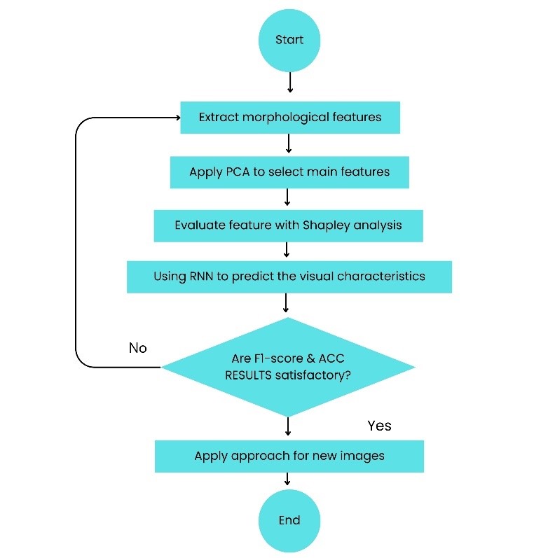
The primary purpose of this study is to classify the normal and disease eyes in correct groups. In this regard, classification is performed on the different varieties of Keratoconus images. This dataset consists of 900 images in two different categories (450 images for Keratoconus and 450 images for normal eyes). The classification is conducted following a selection of essential features using feature selection algorithms. For this purpose, consider a dataset D with N attributes, where each tuple is composed of N values. For each new tuple X, classifier predict that X ∈ Ci if the class Ci has a highest probability condition on X. In several classification phases for keratoconus, the performance of generated findings is evaluated based on classification accuracy, recall, f1-score, ROC curve, and prediction time. Precision is a metric that reflects how accurate is the model, i.e., how many of them are actually positive [23]. In this paper, precision represents the proportion of eyes for which keratoconus was accurately predicted by (11). The recall is the measure which identify true positives (Equation (12)). Thus, for all instances which actually have keratoconus disease, recall calculates how many samples correctly realized as having keratoconus disease. The F1-score is a metric combining false positives and negatives to make a balance between precision and recall [23]. It is a weighted average of the precision and recall. Model is regarded true when the F1-score is 1, and false when the F1-score is 0 (Equation (13)). Finally, accuracy is a common metric for describing the classification performance of a model across all classes. It reflects the proportion of accurate forecasts relative to the total number of predictions (Equation (14)). Flowchart of the proposed approach is presented as Figure 3.
$$\text{Precision} = \frac{TP}{TP + FP} \tag{11}$$
$$\text{Recall} = \frac{TP}{TP + FN} \tag{12}$$
$$F1\text{-score} = 2 \times \frac{\text{Precision} \times \text{Recall}}{\text{Precision} + \text{Recall}} \tag{13}$$
$$ACC = \frac{TP + TN}{TP + FP + TN + FN} \tag{14}$$
Here: TF – are True Positives;
FP – are False Positives;
FN – are False Negatives;
ACC – is acceleration index;
TN – are True Nagatives.
4. Results Discussion
4.1. Dataset
In this regard, 7 morphological features are defies as Table. 2. In order to classify the different varieties of Keratoconus images, the dataset consist of 900 images is considered for this study. The minimum, mean, maximum and standard deviation of morphological features for both types of corneas are given in Table 3.
4.2. PCA-based feature analysis
After extraction of features, PCA is applied to reduce the amount of features, while keeping the almost all of important information from dataset. This method extracts variables which are called principal components (PCs) that are uncorrelated to each other. The obtained result is shown in Figure 4. With using PCA on cornea dataset, The matrix of eigenvectors and eigenvalues are obtained as (15) and (16), respectively.
Table 2: Morphological Features
Feature | Definition |
Area | No. of pixel’s boundaries |
Major Axis Length | Length of longest line on the Keratoconus image |
Minor Axis Length | Length of shortest line on the Keratoconus image |
Eccentricity | Ellipse’s eccentricity with the equal moments |
Convex Area | No. of pixels of the smallest convex cornea |
Extent | Keratoconus’ region vs. total pixels of bounding box |
Perimeter | Distance between boundaries & pixels around of cornea |
Table 3: Statistical data of different features
Feature | Min. | Mean | Max. | Standard Deviation |
Area | 25387 | 87804.1 | 235047 | 39002.11 |
Major Axis Length | 225.63 | 430.93 | 997.292 | 116.035 |
Minor Axis Length | 143.71 | 254.488 | 492.275 | 49.989 |
Eccentricity | 0.349 | 0.782 | 0.962 | 0.09 |
Convex Area | 26139 | 91186.1 | 278217 | 40769.29 |
Extent | 0.38 | 0.7 | 0.835 | 0.053 |
Perimeter | 619.07 | 1165.90 | 2697.76 | 273.764 |
$$A = \begin{bmatrix} 0.448 & -0.116 & 0.005 & -0.111 & -0.611 & -0.100 & -0.624 \\ 0.443 & 0.137 & -0.101 & 0.495 & 0.0876 & -0.686 & 0.228 \\ 0.389 & -0.375 & 0.236 & -0.656 & 0.384 & -0.240 & 0.130 \\ 0.203 & 0.611 & -0.629 & -0.426 & 0.075 & 0.054 & 0.020 \\ 0.451 & -0.0877 & 0.037 & 0.056 & -0.392 & 0.471 & 0.640 \\ -0.056 & -0.667 & -0.731 & 0.109 & 0.057 & 0.023 & -0.002 \\ 0.451 & 0.034 & 0.044 & 0.340 & 0.555 & 0.487 & -0.364 \end{bmatrix} \tag{15}$$
$$\lambda = \begin{bmatrix} 4.838 \\ 1.455 \\ 0.630 \\ 0.057 \\ 0.022 \\ 0.006 \\ 0.001 \end{bmatrix} \tag{16}$$
$$V_j = \frac{\lambda_j}{\sum_{j=1}^{p} \lambda_j}, \quad j = 1,2,\ldots,p \tag{17}$$
$$V_1 = 0.690 \quad V_2 = 0.2076 \quad V_3 = 0.090 \quad V_4 = 0.008 \tag{18} \\ V_5 = 0.003 \quad V_6 = 0.001 \quad V_7 = 0.000$$
$$Z_1 = 0.448X_1 + 0.443X_2 + 0.389X_3 + 0.203X_4 + 0.451X_5 – 0.056X_6 + 0.451X_7 \tag{19}$$
$$Z_2 = -0.116X_1 + 0.137X_2 – 0.375X_3 + 0.611X_4 – 0.088X_5 – 0.667X_6 + 0.034X_7 \tag{20}$$
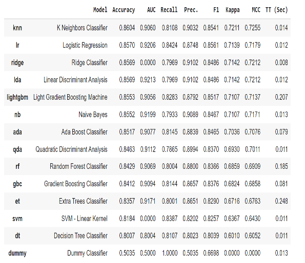
Obtained results for this part is represented in Table 4. After applying PCA, the best result belonged to KNN classifier with accuracy equal to 86.04%. According to results extracted by applying PCA, if the dimension of features reduced from r = 7 to r = 2 then the calculated error was less than 0.5%.
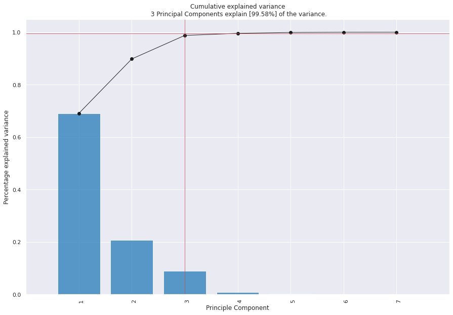
Table 4: Classification models and their statistics after PCA
4.3. Shapley Feature Analysis
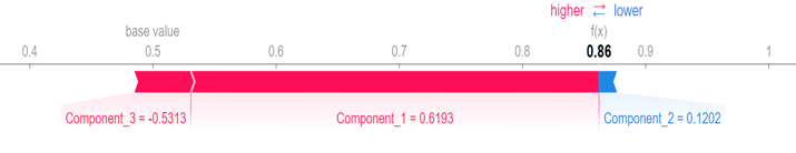
For better assessment, SHAP (Shapley Additive Explanations) is used to explain the most important features by visualizing the output (Figure 5). The first, second and third PCs are considered as component 1, component 2 and component 3, respectively. In this figure, feature values have two colors. Pink is used for features cause increasing and blue is used for showing the features which causes decreasing in prediction. As can be seen in this figure, first PC has the most impressive effect with the longest pink line, and the third PC has the lowest contribution.
4.4. Feature based RNN results
To avoid the disturbance caused by the gradient vectors, long short-term memory (LSTM) activation function has been used in connection with the active nodes in the RNN network.
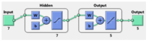
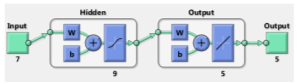
In this situation, according to the input data consist of uncorrected visual acuity, degree of sphere, astigmatism, orientation of astigmatism and best corrected visual acuity, the LSTM activation function adapt the input and by considering the transient state value, it scales the output of the activation function. To determine the optimal value of weight coefficient, stochastic gradient descent method has been used. This proposed approach has 6 layers. The first layer is the input layer and the second and third layers are used as LSTM layers. In the fourth layer, two actions are performed. In the first stage, the output of the third layer is connected with the input vector, and in the next stage, a linear combination of the inputs is produced in each time step. The fifth and sixth layers include a multilayer perceptron neural network. A hidden layer is embedded in this network. The complete specifications of the proposed method are listed in Table 5.
The output of the neural networks are the five characteristics of eye vision. The RNN used in this research is a neural network with 44 hidden neurons in hidden layer. From the available data, 85% were used for training and the rest for evaluation and validation of each of the trained networks. By comparing the coefficient of cell size changes in the two groups of keratoconus patients and the group of healthy individuals, no significance difference was found (P = 0.828). By examining the specular microscopy images, changing the shape of the cells, people with keratoconus only in seven eyes (9.26%) and in the control group, it was seen only in six eyes (24%). According to the amount of ratio equal to 1.1, the chance of cell shape change in the corneal endothelium of patients with keratoconus was 10% higher than that of healthy individuals. According to the confidence interval of 0.95 which was calculated between 0.59 – 1.095, it can be said that the cell shape change in the corneal endothelium of these two cases and control groups was similar to each other. Since by comparing the average cell density in two groups of keratoconus patients and healthy individuals (control group), no significant statistical difference was seen as equal to P = 0.96. The cell density in the upper part of the cornea is the highest in the two groups, but the interaction of the group (being sick or healthy) on the cell density was not significant (P = 0.96) (Table 5).
Table 5: Characteristics of the RNN method
No. of | 900 | Type of | RNN + LSTM |
Hidden | 44 | Function of | Log – Sigmoid |
Coefficient optimizer | Stochastic | Function of | Tan – Sigmoid |
Table 6: Comparison of the average difference in cell density
of different areas of the cornea
Region 1 | Region 2 | Mean of difference | Sig. |
Central | Superior | -335.3 | 0.000 |
Inferior | -28.9 | 0.994 | |
Nasal | -24.1 | 0.997 | |
Temporal | -107.5 | 0.529 | |
Superior | Central | 335.3 | 0.000 |
Inferior | 306.4 | 0.000 | |
Nasal | 311.2 | 0.000 | |
Temporal | 227.8 | 0.010 | |
Inferior | Central | 289 | 0.994 |
Superior | -306.4 | 0.000 | |
Nasal | 4.8 | 1.000 | |
Temporal | -78.6 | 0.787 | |
Nasal | Central | 24.1 | 0.997 |
Superior | -311.2 | 0.000 | |
Inferior | -4.8 | 1.000 | |
Temporal | -83.4 | 0.748 | |
Temporal | Central | 107.5 | 0.529 |
Superior | -227.8 | 0.010 | |
Inferior | 78.6 | 0.787 | |
Nasal | 83.4 | 0.748 |
4.4.1. Scenario 1: 6 months after Keraring operation
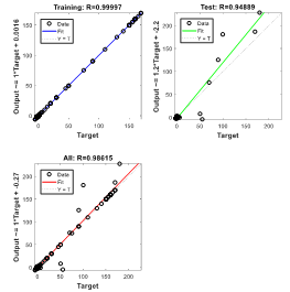
In predicting the visual characteristics of eyes with keratoconus six months after keraring implantation with the help of RNN, the regression result of training data is obtained as equal to RTraining = 0.99997. It implies a very close proximity between output values and network objectives in the training set (Figure 6). In the graph labeled Test, the regression analysis of the evaluation data set is presented. For evaluation data and for all data, the regression value is equal to RTest = 0.94889 and RAll = 0.98615, respectively.
4.4.2. Scenario 2: 12 months after Keraring operation
For predicting the visual characteristics of the keratoconus after twelve months of keraring ring implantation, special RNN structure is designed (Figure 7). The regression of training data is RTraining = 0.99992, which indicates a very close proximity of the network’s outputs to goals in the training set. In the evaluation level, the regression value is obtained as RTest = 0.92344 and for all data, the regression value is calculated as RAll = 0.98165.
(Scenario 1)
4.4.3. Scenario 3: 6 months after Myoring
In predicting As can be seen in Figure 8, in predicting the visual characteristics of eyes with keratoconus six months after myoring ring implantation using the RNN, the regression for training data is RTraining = 0.99881. Also, in the graph of the relationship between the output and the target, the fitted line has an angle close to 45 which indicates the high similarity between the outputs and the targets in the training set. The regression value for evaluation data is RTest = 0.92021 and for all data RAll = 0.98237 which is close to unit (perfect match).
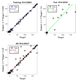
(6 months after Myoring)
4.4.4. Scenario 4: 12 months after Myoring
For predicting the visual characteristics of eyes with keratoconus complications twelve months after myoring ring implantation, special RNN structure has been used (Figure 9). The training data set, has a regression of RTraining = 0.99968 and for the evaluation data, the regression value is RTest = 0.90891. From the regression analysis for all data (training and evaluation), RAll = 0.95364 was obtained.
4.5. Results Comparison
In this section, the results of the proposed method are compared with KerNet, LeNet and AlexNet. In the first stage, the training accuracy versus number of features for different methods are compared with each other and the results obtained are shown in Figure 9. As can be seen, as the number of features increases, the accuracy of the obtained results decreases for all methods. At the same time, the proposed approach brought the least amount of accuracy reduction and this indicates that by increasing the number of features, using the proposed approach provides valuable results.
By selecting 100 features, the accuracy of the proposed approach is more than 94%. This dedicates that the designed approach has less sensitivity to the increase in the number of features than other traditional methods and so, the proposed approach can easily be used for problems on larger scales. In the following, criteria including Precision, Recall, F1-score and ACC have been used to compare the methods. The results of comparison are shown in Table 6.
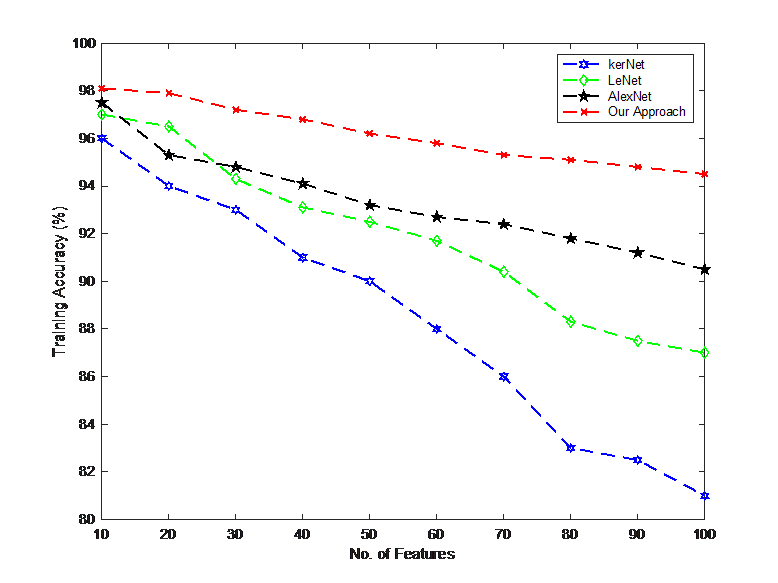
Table 7: Comparison of different metrics between methods
Model | Evaluation Metrics (%) | |||
ACC | Recall | Precision | F1-Score | |
Our Approach | 94.83 | 94.15 | 95.07 | 94.14 |
KerNet | 94.74 | 93.71 | 94.10 | 93.89 |
LeNet | 83.63 | 81.02 | 82.27 | 80.94 |
AlexNet | 92.40 | 90.66 | 91.64 | 91.08 |
5. Conclusion
Keratoconus disease in mild and moderate stages has an effect on cell density, change in cell shape and endothelium. The most advanced available treatment for this disease is intracorneal ring implantation surgery. This surgery is used in very advanced cases of the disease or in some mild to moderate hunchbacks where it is not possible to use contact lenses due to the shape of the cornea. Considering that the success rate of the surgery in keratoconus patients are different and if the treatment is unsuccessful, the patient will need a corneal transplant. One of the concerns of ophthalmologists is which of the patients is a good candidate for this surgery and for whom this method brings better visual results. For this purpose, 900 images of Cornea were used and 7 morphological features were defined. These features consist of Area, Major Axis Length, Minor Axis Length, Convex Area, Perimeter, Eccentricity & Extent. For feature extraction Principal Component Analysis as well as three classification methods including logistics regression (LR), k-nearest neighbors (KNN) and decision tree (DT) algorithms were used. At the principal component analysis (PCA) stage, the contribution of different PCs were determined. Based on it’s results, the first PC had a contribution of more than 69%, the variance of the first two PCs was about 89%. Hence, the feature dataset could be reduced from 7 to 2.
For comparison the results of different methods, 810 samples were used for determination of models’ parameters and the rest of them were preserved for prediction accuracy analysis. In the next part, the obtained results from applying different classification methods such as LR, KNN and DT on original dataset were compared to each other. By the results, the logistic regression (LR) had the best performance with 88.52% accuracy. After applying PCA method based on first two PC, the best accuracy belonged to KNN method (more than 86%). In the last part of this paper, SHAP (Shapley Additive Explanations) was used to more explain the most important features by visualizing the output. the corneal topography is used as an input to a recurrent neural network (RNN) to identify whether or not the patient has keratoconus. By refining the settings of the RNN, the test set accuracy of the proposed technique was enhanced to 99.33%. Based on the obtained results, the average prediction error of the visual characteristics of a patient with keratoconus six and twelve months after the Kraring ring implantation using RNNs with eight and seven neurons in the hidden layer is calculated as 9.82% and 9.29%, respectively. In order to predict the visual characteristics of a patient six and twelve months after Myoring ring implantation, RNNs with five and nine neurons in the hidden layer were used, and the average error of estimating characteristics was calculated as 11.46%, and 7.47%, respectively.
Conflict of Interest
The authors declare no conflict of interest.
- J. Santodomingo-Rubido, G. Carracedo, A. Suzaki, C. Villa-Collar, S. J. Vincent, “Keratoconus: An updated review,” Contact Lens and Anterior Eye, vol. 45, no. 3, 101559, 2022, doi.org/10.1016/j.clae.2021.101559.
- A. Lavric, and P. Valentin, “KeratoDetect: keratoconus detection algorithm using convolutional neural networks.”, Computational intelligence and neuroscience, 2019, doi.org/10.1155/2019/8162567.
- M. M. Vandevenne et al., “Artificial intelligence for detecting keratoconus”, Cochrane Database of Systematic Reviews 11, 2023, doi.org/10.1002/14651858.CD014911.pub2.
- V. Galvis, T. Sherwin, A. Tello, J. Merayo, R. Barrera, and A. Acera, “Keratoconus: an inflammatory disorder?.” Eye 29, no.7, 2015, 843-859, doi.org/10.1038/eye.2015.63.
- M.J. Kaisania, “A machine learning approach for keratoconus detection.” (Ph. D Thesis, 2021).
- P. J. Shih, H. J. Shih, I. J. Wang, and S. W. Chang. “The extraction and application of antisymmetric characteristics of the cornea during air-puff perturbations,” Computers in Biology and Medicine, no. 168, 107804, 2024, doi.org/10.1016/j.compbiomed.2023.107804.
- M. F. Greenwald, B. A. Scruggs, J. M. Vislisel, and M. A. Greiner. ”Corneal imaging: an introduction.” Iowa City (Iowa): Department of Ophthalmology and Visual Sciences, University of Iowa Health Care 9, 2016.
- A., H. Alyaa, H. N. Ghaeb, and Z. M. Musa. ”Support vector machine for keratoconus detection by using topographic maps with the help of image processing techniques.” IOSR Journal of Pharmacy and Biological Sciences, vol. 12, no. 6, 2017, 50-58, doi.org/10.9790/3008-1206065058.
- M. C. Arbelaez, F. Versaci, G. Vestri, P. Barboni, and G. Savini. ”Use of a support vector machine for keratoconus and subclinical keratoconus detection by topographic and tomographic data.” Ophthalmology vol. 119, no. 11, 2012, 2231-2238, doi.org/10.1016/j.ophtha.2012.06.005.
- A. Lavric, P. Valentin, T. Hidenori, and S. Yousefi. ”Detecting keratoconus from corneal imaging data using machine learning.” IEEE Access vol. 8, 2020, 149113-149121, doi.org/10.1109/ACCESS.2020.3016060.
- K. Kamiya, Y. Ayatsuka, Y. Kato, F. Fujimura, M. Takahashi, N. Shoji, Y. Mori, and K. Miyata. “Keratoconus detection using deep learning of colour-coded maps with anterior segment optical coherence tomography: a diagnostic accuracy study.” BMJ open vol. 9, no. 9, 2019, doi.org/10.1136/bmjopen-2019-031313.
- L. M. Hartmann et al., “Keratoconus Progression Determined at the First Visit: A Deep Learning Approach With Fusion of Imaging and Numerical Clinical Data,” Translational Vision Science & Technology, vol. 13, no. 5, 2024, doi.org/10.1167/tvst.13.5.7
- A. Tillmann et al., “Acute corneal melt and perforation – a possible complication after riboflavin/UV-A crosslinking (CXL) in keratoconus.,”American journal of ophthalmology case reports, vol. 28, 101705, 2022, doi.org/10.1016/j.ajoc.2022.101705
- A. H. Al-Timemy, N. H. Ghaeb, Z. M. Mosa, and J. Escudero. “Deep transfer learning for improved detection of keratoconus using corneal topographic maps.” Cognitive Computation vol.14, no. 5, 2022, 1627-1642. doi.org/10.1007/s12559-021-09880-3
- K. Kazutaka, Y. Ayatsuka, Y. Kato, N. Shoji, Y. Mori, and K. Miyata. “Diagnosability of keratoconus using deep learning with Placido disk-based corneal topography. ” Frontiers in Medicine vol. 8, 2021, 724902, doi.org/10.3389/fmed.2021.724902
- I. Issarti, A. Consejo, M. Jiménez-García, S. Hershko, C. Koppen, and J. J. Rozema. “Computer aided diagnosis for suspect keratoconus detection. ” Computers in biology and medicine vol. 109, 2019, 33-42. doi.org/10.1016/j.compbiomed.2019.04.024
- B. R. Salem, and V. I. Solodovnikov. “Decision support system for an early-stage keratoconus diagnosis. ” In Journal of Physics: Conference Series, vol. 1419, no. 1, p. 012023. IOP Publishing, 2019, doi.org/10.1088/1742-6596/1419/1/012023
- X. Xu, T. Liang, J. Zhu, D. Zheng, and T. Sun. “Review of classical dimensionality reduction and sample selection methods for large-scale data processing,” Neurocomputing, vol. 328, 2019, 5-15, doi.org/10.1016/j.neucom.2018.02.100
- H. S. Hippert, C. E. Pedreira, and R. C. Souza. “Neural networks for short-term load forecasting: A review and evaluation,” IEEE Transactions on power systems vol. 16, no. 1, 2001, 44-55, doi.org/10.1109/59.910780
- E. Mocanu, P. H. Nguyen, M. Gibescu, and W. L. Kling. ”Deep learning for estimating building energy consumption. “Sustainable Energy, Grids and Networks 6, 2016, 91-99, doi.org/10.1016/j.segan.2016.02.005
- M. R. Arahal, A. Cepeda, and E. F. Camacho. ”Input variable selection for forecasting models. “ IFAC Proceedings, Vol. 35, no. 1, 2002, 463-468, doi.org/10.3182/20020721-6-ES-1901.00730
- Fan, Cheng, Fu Xiao, and Yang Zhao. “A short-term building cooling load prediction method using deep learning algorithms. ”Applied energy vol. 195, 2017, 222-233, doi.org/10.1016/j.apenergy.2017.03.064
- S. Hochreiter, and J. Schmidhuber. “Long short-term memory. ” Neural computation vol. 9, no. 8, 1997, 1735-1780, doi.org/10.1162/neco.1997.9.8.1735