information about soil properties help the farmers to do effective and efficient farming, and yield mo . An attempt has been made in this paper to predict the soil properties using machine learning approaches. The main properties of soil prediction are Calcium, Phosphorus, pH, Soil Organic Carbon, and Sand. These properties greatly affect the production of crops. Four well-known machine learning models, namely, multiple linear regression, random forest regression, support vector machine, and gradient boosting, are used for prediction of these soil properties. The performance of these models is evaluated on Africa Soil Property Prediction dataset. Experimental results reveal that the gradient boosting outperforms the other models in terms of coefficient of determination. Gradient boosting is able to predict all the soil properties accurately except phosphorus. It will be helpful for the farmers to know the properties of the soil in their particular terrain.

1. Introduction

India has a 1.27 billion population, which is second-most in the entire world. It is the seventh-largest country in the world with an area of 3.288 million sq km. Indians are very much dependent on agriculture. It is the largest source of livelihood in India. In rural households, 70% of people are primarily dependent on agriculture, with about 82% of farmers being small and marginal. In 2020-21, total food grain production was estimated at 308.65 million tonnes (MT). India is the largest producer (25% of global produc- tion), the consumer (27% of world consumption), and the importer (14%) of pulses in the world. India’s annual milk production was 165 MT (2017-18), making India the largest producer of milk, jute, and pulses, with the world’s second- largest cattle population of 190 million in 2012 [1]. With merely 2.4% arable land resources and 4% water resources [2], Indian agriculture is feeding nearly 1.3 billion people, which implicates huge pressure on land and other natural resources for continuous productivity [3].

After the green revolution(which started in the 1960s), India made significant progress in agriculture production, which became possible due to modernization. With the development in technology, farmers have been provided with advanced farming techniques, better seeds (High Yielding Variety(HYV) seeds), mechanized farm tools, chemical fertilizers, facilities of irrigation, and electrical energy[4]. Since the green revolution, there has been excessive use of chemical fertilizers which has increased the crop productivity manifold. However, it has turned into a problem as overuse of these chemical fertilizers has been detrimental for crop productivity and soil fertility. Fertilizer recommendations rarely match soil needs which has caused overuse of these chemical products[3].

So, there is a need for accurate fertilizer recommendations for the farmer and accurately analyzing soil properties is the first step for that. Indian Agricultural Research Institute(ICAR) recommends soil test-based, balanced and integrated nutrient management through conjunctive use of both inorganic and organic sources of plant nutrients to reduce the use of chemical fertilizers, preventing deterioration of soil health, environment and contamination of groundwater [5].

This paper aims to study the ability of various machine learning techniques to accurately predict the soil proper- ties relevant for agriculture using spectroscopy data. Over the last 20 years, soil spectroscopy has become a powerful technique for analyzing relative to the traditionally used chemical methods, particularly in the infrared range. Spectroscopy is known as a fast, economical, quantitative, and eco-friendly technique, which can be used in the fields as well as in the laboratory to provide hyperspectral data with narrow and numerous data [6], [7]. In this paper, the different properties of soil like Calcium, Phosphorus, pH, Soil Organic Carbon and Sand are predicted by using machine learning models. In [8], it is found consistently higher performance of machine learning methods over simpler approaches in spectroscopy. In [9], it is reported the decline in the use of some models such as Support Vector Machines (SVM) and multivariate adaptive regression spline, giving way to more advanced alternatives such as Random Forest (RF). In this paper, machine learning algorithms such as Multivariate Regression, Random Forest Regression, Support Vector Machine, and Gradient boosting with a different degree of accuracy are used for comparative analysis. The dataset is split into a training and testing dataset (80% training data and 20% testing data) [10]. The machine learning models are trained on the training data. After a model is trained, the testing data is used to check the accuracy of the trained model. Here, the coefficient of determination (COD) is calculated to check the working of the models after being trained. After training the models, the best working model is deployed to predict the properties of the soil (Calcium, Phosphorous, pH, Soil Organic Carbon, and Sand). These predicted values of the soil properties are going to be helpful in choosing the different suitable fertilizers.

The remaining structure of this paper is as follows. Section 2 presents the materials and methods used for soil prediction. Experimental results and discussion are mentioned in Section 3. Section 4 presents the concluding remarks.

2. Materials and Methods

In this section, the dataset and techniques used for soil prediction are briefly described.

2.1. Data Set

A collection of 1,886 soil sample measures is used for performance comparison of machine learning models. The soil was collected from a variety of locations in Africa. Each data point consists of 3,594 features :

1. PIDN: unique soil sample identifier
2. SOC: Soil organic carbon
3. pH: pH values
4. Ca: Mehlich-3 extractable Calcium
5. P: Mehlich-3 extractable Phosphorus
6. Sand: Sand content
7. 96 – m599.76: There are 3,578 mid-infrared absorbance measurements. For example, the ”m599.76” column is the absorbance at wavenumber 599.76 cm-1.
8. Depth: Depth of the soil sample (2 categories: ”Topsoil”, 2. ”Subsoil”)
9. BSA: Average long-term Black Sky Albedo measurements from MODIS satellite images (BSAN = near- infrared, BSAS = shortwave, BSAV = visible)
10. CTI: Compound topographic index calculated from Shuttle Radar Topography Mission elevation data
11. ELEV: Shuttle Radar Topography Mission elevation data
12. EVI: Average long-term Enhanced Vegetation Index from MODIS satellite images
13. LST: Average long-term Land Surface Temperatures from MODIS satellite images (LSTD=day time temper- ature, LSTN night time temperature)
14. Ref: Average long-term Reflectance measurements from MODIS satellite images (Ref1 = blue, Ref2 = red, Ref3 = near-infrared, Ref7 = mid-infrared)
15. Reli: Topographic Relief calculated from Shuttle Radar Topography mission elevation data
16. TMAP TMFI: Average long-term Tropical Rainfall Monitoring Mission data (TMAP = Mean Annual Precipitation, TMFI = Modified Fournier Index)

The five main target variables for predictions are: Soil Organic Carbon(SOC), pH, Calcium, Phosphorus, and Sand. The data has not been altered and is in the original measurements. Thus, it includes both positive as well as negative values. The dataset was available at Kaggle.com under a competition named ”Africa Soil Property Prediction Com- petition” [11].

2.2. Techniques Used

2.2.1. Linear Regression

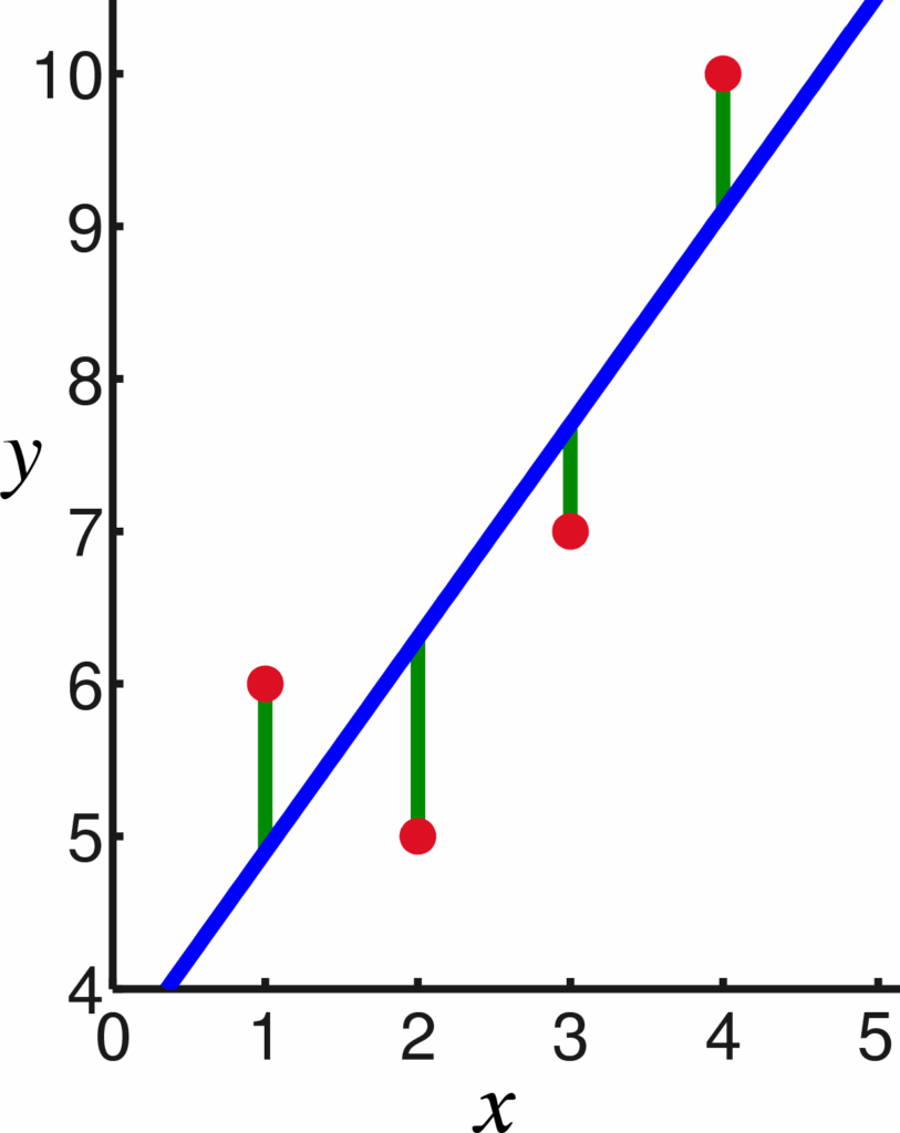
Regression is an approach to supervised learning. It can be used to model continuous variables or make predictions. Some examples of application of linear regression algorithm are: prediction of the price of real estate, forecasting of sales, prediction of students’ exam scores, forecasting of movements in the price of a stock in the stock exchange. In Regression, we have the labeled datasets and the output variable value is determined by input variable values. The most simple form of regression is linear regression where the attempt is made to fit a straight line (straight hyper- plane) to the dataset and it is possible when the relationship between the variables of the dataset is linear as shown in Figure 1

Advantage of linear regression is, that it is easy to understand and it is also easy to avoid overfitting by regularization. SGD is used to update linear models with new data. Linear Regression is a good fit if it is known that the relationship between covariates and response variables is linear.

It shifts focus from statistical modeling to data analysis and preprocessing. Linear Regression is good for learning about the data analysis process. However, it is not a recommended method for most practical applications because it oversimplifies real-world problems [12]-[14].

2.2.2. Multiple Linear Regression

A simple linear regression model has a dependent variable guided by a single independent variable. However, real-life problems are more complex. Generally, one dependent variable depends on multiple factors. For example, the price of a house depends on many factors like the neighborhood it is situated in, it’s area, number of rooms, attached facilities, availability of nearby facilities like airport/railways/shopping centres, etc. In simple linear regression, there is a one-to-one relationship between the input variable and the output variable. But in multiple linear regression, there is a many-to-one relationship between a number of independent (input/predictor) variables and one dependent (output/response) variable. Adding more input variables does not mean the regression will be better or will offer better predictions.

This technique gives a deep insight into the relationship between the set of independent variables and dependent variables. It also gives insight into relationships among the independent variables. This is achieved through multiple regression, tabulation techniques, and partial correlation. It models complex real-world problems in a practical and realistic way.

However, it suffers from high computational complexity, requires knowledge and expertise on statistical techniques and statistical modeling. The sample size for statistical modeling needs to be high to get a higher confidence level on analysis outcome. Also, it often gets too difficult to do a meaningful analysis and interpretation of the outputs of the statistical model [12]–[14].

2.2.3. Decision Tree

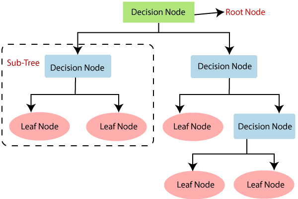
A Decision Tree is a Supervised Machine Learning approach to solve classification and regression problems by continuously splitting data based on a certain parameter. The decisions are in the leaves and the data is split in the nodes as shown in Figure 2. In the Classification Tree, the decision variable is categorical (outcome in the form of Yes/No) and in the Regression tree, the decision variable is continuous. Decision Tree is suitable for regression as well as classification problems. It offers ease in interpretation, handles categorical and quantitative values, is capable of filling missing values in attributes with the most probable value and assures a high performance due to efficiency of the tree traversal algorithm. Decision Tree might encounter the problem of overfitting for which Random Forest is the solution which is based on an ensemble modeling approach[15]. Disadvantages of decision tree are: unstable, difficult to control size of the tree, prone to sampling error and locally optimal solution. Decision Trees can be used in predicting the future use of library books and tumor prognosis problems [12].

2.2.4. Random Forest

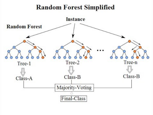
Random forests or random decision forests is an ensemble learning method for classification, regression, and other tasks that operate by constructing a multitude of decision trees at training time. For classification tasks, the output of the random forest is the class selected by most trees. For regression tasks, the mean or average prediction of the individual trees is returned as shown in Figure 3. Random decision forests correct for decision tree’s habit of overfitting to their training set. Random forests generally outperform decision trees, but their accuracy is lower than gradient boosted trees. However, data characteristics can affect their performance [16]–[18].

2.2.5. Gradient Boosting

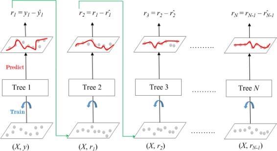
Gradient boosting is used in regression and classification tasks. It gives a prediction model in the form of an ensemble of weak prediction models, which are typically decision trees as shown in Figure 4. When a decision tree is a weak learner, the resulting algorithm is called gradient-boosted trees; it usually outperforms random forest. A gradient- boosted model is built in a stage-wise fashion, as in other boosting methods, but it generalizes the other methods by allowing optimization of an arbitrary differential loss function [19] [18]

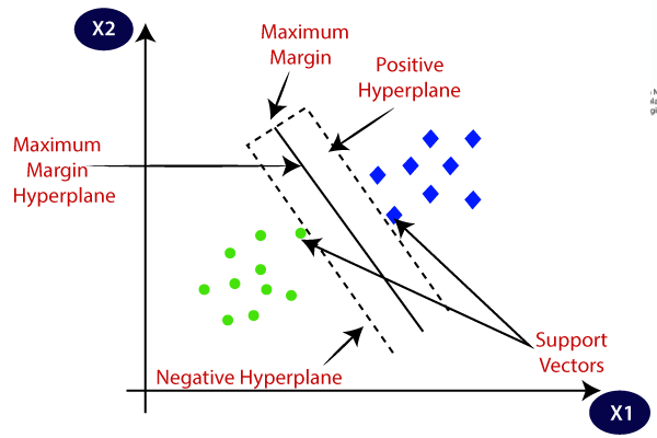
2.2.6. Support Vector Machine

Support Vector Machine (SVM) is a supervised learning model, which can be used for both classification and regression. It is a non-probabilistic binary linear classifier. It was developed in 1993 at Bell laboratories. It is one of the most robust learning frameworks. SVM maps training samples into a sample space to maximize the width between two categories. New samples are mapped to a space and they are classified on the base of which side of the gap they are, as shown in Figure 5 [20].

2.3. Methodology used for soil prediction

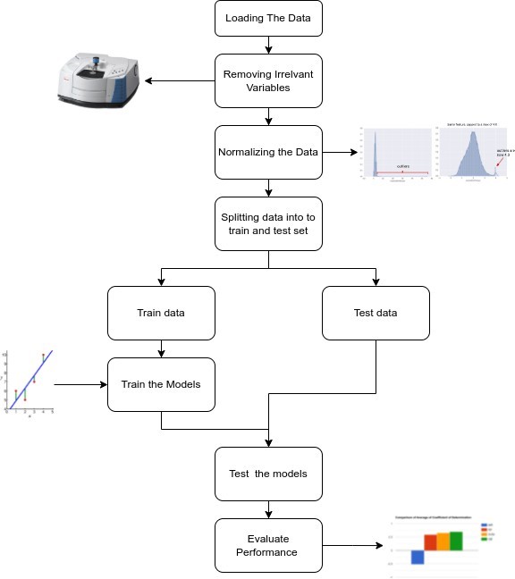
2.3.1. Preparing the data

1. Removing irrelevant variables : Removing the un- necessary/irrelevant variables like PIDN are removed during the preprocessing These variables in the data set might lead to the model not working properly due to a possible false correlation
2. Normalizing data : Normalization is a technique of- ten applied as part of data preparation for machine learning. The goal of normalization is to change the values of numeric columns in the data set to use a common scale without distorting differences in the ranges of values or losing information. Normalization is also required for some algorithms to model the data correctly. For eg. assume your input data set contains one column with values ranging from 0 to 1, and another column with values ranging from 10,000 to 100,000. The great difference in the scale of the numbers could cause problems when you attempt to combine the values as features during modeling. Normalization avoids these problems by creating new values that maintain the general distribution and ratios in the source data, while keeping values within a scale applied across all numeric columns used in the data set.
3. Splitting data into train and test sets : The train-test split procedure is used to estimate the performance of machine learning They are used to make predictions on data. It is a fast and easy procedure to perform, the results of which allow you to compare the performance of machine learning algorithms for your predictive modeling problem. Although it is simple to use and interpret. Some classification problems do not have a balanced number of examples for each class label. As such, it is desirable to split the dataset into train and test sets in a way that preserves the same proportions of examples in each class as observed in the original dataset.

3. Results and Discussion

In this section, the performance evaluation of machine learning models is evaluated.

3.1. Performance measure

Coefficient of determination as metric is used for comparing the performance of different machine learning models trained on the same data set. In statistics, the coefficient of determination(𝑅² or 𝑟² and pronounced “R squared”), is the proportion of the variation in the dependent variable that is predictable from the independent variable(s). The formula is defined as [21]:

Where 𝑅𝑆𝑆 represents sum of squares residuals and 𝑇𝑆𝑆 represents Total sum of squares.

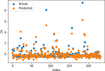
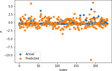
Table 1: Multivariate Regression Coefficient of Determination

3.2. Multiple Linear Regression

Figures 7-11 depict the actual and predicted values of soil properties using multiple linear regression. It is observed from the figures that the predicted values attained from multiple linear regression are almost similar to the actual values for calcium and soil carbon. Table 1 shows the results obtained from multiple linear regression. The results reveal that the value of the coefficient of determination is higher for calcium and carbon.

3.3. Random Forrest Regression

Figures 12-16 show the actual and predicted values of soil properties using random forest. It can be found from the figures that the predicted values attained from random forest are almost similar to the actual values for calcium, sand, and soil carbon. Table 2 represents the values of coefficient of determination obtained from random forest. The results reveal that the value of coefficient of determination is higher for calcium, carbon, and sand.

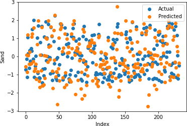
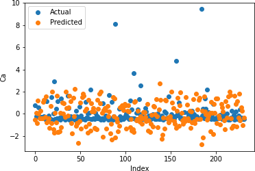
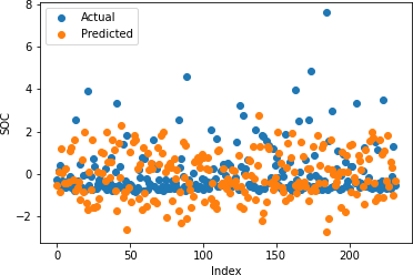
Table 2: Random Forrest Regression Coefficient of Determination

3.4. Support Vector Machine Regression

Figures 17-21 illustrate the actual and predicted values of soil properties using support vector machine. These figures reveal that the predicted values attained from support vector machine are almost similar to the actual values for calcium, sand, pH, and soil carbon. Table 3 represents the values of the coefficient of determination obtained from support vector machine. The results reveal that the value of the coefficient of determination is higher for calcium, carbon, pH, and sand.

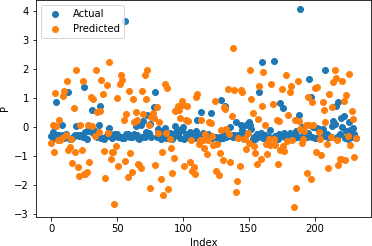
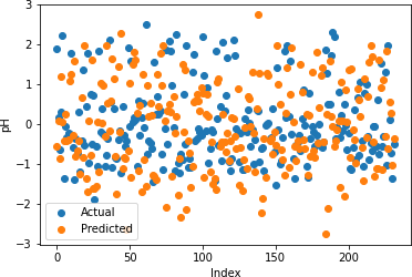
Table 3: Support Vector Regression Coefficient of Determination

3.5. Stochastic Gradient Boosting Regression

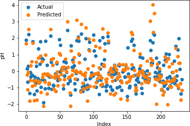
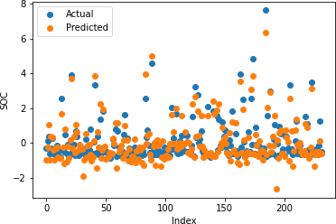
Figures 22-26 show the actual and predicted values of soil properties using gradient boosting. These figures reveal that the predicted values attained from gradient boosting are almost similar to the actual values for calcium, sand, pH, and soil carbon. Table 4 represents the values of the coefficient of determination obtained from gradient boost- ing. The results reveal that the value of the coefficient of determination is higher for calcium, carbon, pH, and sand.

Table 4: Gradient Boosting Coefficient of Determination

3.6. Discussion

Table 5: Comparative analysis of machine learning model in terms of Coefficient of Determination

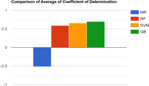
Table 6: Average performance obtained from different machine learning models

In Table 5 MR is Multiple Linear Regression, RF is random forest regression, SVM is Support Vector Machine regression and GB is gradient boosting regression. Here we are comparing the performance of each technique in predicting an individual component in soil.

Table 5 shows the performance comparison of four machine learning models in terms of the Coefficient of determination for every component of soil. The results reveal that gradient boosting performs better than others in terms of C, SOC, and Sand. Table 6 depicts the average performance of machine learning models. It is observed from the table that gradient boosting outperforms the others in terms of the Coefficient of determination.

We find that there is very little correlation of the spectroscopy data and remote sensing data with the with the amount of phosphorous in the soil, even being negative in case of multiple linear regression and random forest. While both gradient boosting and support vector machines give a very weak positive correlation. Possible ways to fix this problem is either getting more data or trying out deep learning techniques. Gradient boosting outperforms all other methods in Predicting calcium, soil organic carbon and sand, while coming at a close second in predicting pH. In a real world deployment, a hybrid approach can be used for evaluating each component. Also, there’s a possibility of creating hybrid models that use consensus of multiple models. This can be done by taking weighted averages of output of different models may mitigate problem of over fitting and improve accuracy.

4. Conclusion

This paper studied the machine learning techniques to predict soil properties for precision agriculture. Four machine learning techniques were used to evaluate the soil properties such as Calcium, Phosphorus, pH, Soil Organic Carbon, and Sand. These techniques were trained and tested on the Africa Soil Property Prediction dataset. It is observed from the results that stochastic gradient boosting performed better than the other techniques. Stochastic gradient boosting was able to predict Phosphorous better than multiple linear regression and Random Forest. Support vector regression was best at predicting the phosphorous component.

It can be seen that there is a potential to use spectroscopy as an alternative method of soil component analysis. Deep learning and hybrid models may be used for predicting soil properties in an effective and efficient manner. The main limitation of our study is the use a small number of soil components for prediction. This study can be extended by using a large dataset and other models.

1. O. Food, of United Nations, “India at a glance”, https://www.fao. org/india/fao-in-india/india-at-a-glance/en/.
2. v. B. Ephraim Nkonya, Alisher Mirzabaev, Economics of Land Degrada- tion and Improvement – A Global Assessment for Sustainable Development, Spinger, 2016.
3. S. B. Arun Kumar, A. Kumar, “Prospective of Indian agricul- ture: highly vulnerable to huge unproductivity and unsustainabil- ity”, CURRENT SCIENCE, vol. 119, no. 7, pp. 1079–1080, 2020, doi: http://dx.doi.org/10.1002/andp.19053221004.
4. Yadav, “Agricultural situation in india”, 2014.
5. of Agriculture, “Overuse of fertilizer”, https://pib.gov.in/ Pressreleaseshare.aspx?PRID=1696465.
6. Barra, S. Haefele, R. Sakrabani, F. Kebede, “Soil spectroscopy with the use of chemometrics, machine learning and pre-processing tech- niques in soil diagnosis: Recent advances -a review”, TrAC Trends in Analytical Chemistry, vol. 135, 2020, doi:10.1016/j.trac.2020.116166.
7. Patra, R. Pal, P. Rajamani, P. Surya, “Mineralogical composi- tion and c/n contents in soil and water among betel vineyards of coastal odisha, india”, SN Applied Sciences, vol. 2, 2020, doi: 10.1007/s42452-020-2631-5.
8. Barra, S. M. Haefele, R. Sakrabani, F. Kebede, “Soil spectroscopy with the use of chemometrics, machine learning and pre-processing techniques in soil diagnosis: Recent advances–a review”, TrACstry, vol. 135, p. 116166, 2021, doi:https:6/j.trac.2020.116166.
9. Yu, D. Liu, G. Chen, B. Wan, S. Wang, B. Yang, “A neural network ensemble method for precision fertilization modeling”, Mathemat- ical and Computer Modelling, vol. 51, no. 11, pp. 1375–1382, 2010, doi:https://doi.org/10.1016/j.mcm.2009.10.028, mathematical and Computer Modelling in Agriculture.
10. Sydorenko, “Training data”, https://labelyourdata.com/ articles/machine-learning-and-training-data, 2021.
11. “Africa soil property prediction challenge”, https://www.kaggle. com/c/afsis-soil-properties/data.
12. Ray, “A quick review of machine learning algorithms”, “2019 International Conference on Machine Learning, Big Data, Cloud and Parallel Computing (COMITCon)”, pp. 35–39, 2019, doi:10.1109/ COMITCon.2019.8862451.
13. A. Freedman, Statistical Models: Theory and Practice, Cambridge University Press, 2 ed., 2009, doi:10.1017/CBO9780511815867.
14. Yan, Linear Regression Analysis: Theory and Computing, World Scien- tific Publishing Company Pte Limited, 2009.
15. Wu, V. Kumar, J. R. Quinlan, J. Ghosh, Q. Yang, H. Motoda, G. J. Mclachlan, A. Ng, B. Liu, P. S. Yu, et al., “Top 10 algorithms in data mining”, Knowledge and Information Systems, vol. 14, no. 1, p. 1–37, 2007, doi:10.1007/s10115-007-0114-2.
16. K. Ho, “Random decision forests”, “Proceedings of 3rd Interna- tional Conference on Document Analysis and Recognition”, vol. 1, pp. 278–282 vol.1, 1995, doi:10.1109/ICDAR.1995.598994.
17. K. Ho, “The random subspace method for constructing decision forests”, IEEE Transactions on Pattern Analysis and Machine Intelligence, vol. 20, no. 8, pp. 832–844, 1998, doi:10.1109/34.709601.
18. Hastie, J. Friedman, R. Tisbshirani, The Elements of statistical learning: data mining, inference, and prediction, Springer, 2017.
19. M. Piryonesi, T. E. El-Diraby, “Data analytics in asset manage- ment: Cost-effective prediction of the pavement condition index”, Journal of Infrastructure Systems, vol. 26, no. 1, p. 04019036, 2020, doi:10.1061/(asce)is.1943-555x.0000512.
20. Cortes, V. Vapnik, “Support-vector networks”, Machine Learning, vol. 20, no. 3, p. 273–297, 1995, doi:10.1007/bf00994018.
21. N. J.Nagelkerke, et al., “A note on a general definition of the coefficient of determination”, Biometrika, vol. 78, no. 3, pp. 691–692, 1991.

Citations by Dimensions

Citations by PlumX

Crossref Citations

This paper is currently not cited.

No. of Downloads per Month

No. of Downloads per Country