2D HumanPose Estimation (2D-HPE) has been widely applied in many practical applications in life su ction, human-robot interaction, using Convolutional Neural Networks (CNNs), which has achieved many good results. In particular, the 2D-HPE results are intermediate in the 3D Human Pose Estimation (3D-HPE) process. In this paper, we perform a study to compare the results of 2D-HPE using versions of Residual Network (ResNet/RN) (RN-10, RN- 18, RN-50, RN-101, RN-152) on HUman 3.6M Dataset (HU-3.6M-D). We transformed the original 3D annotation data of the Human 3.6M dataset to a 2D human pose. The estimated models are fine-tuning based on two protocols of the HU-3.6M-D with the same input parameters in the RN versions. The best estimate has an error of 34.96 pixels with Protocol #1 and 28.48 pixels with Protocol #3 when training with 10 epochs, increasing the number of training epochs reduces the estimation error (15.8 pixels of Protocol #3). The results of quantitative evaluation, comparison, analysis, and illustration in the paper.

1. Introduction

Human pose estimation is defined as the process of localizing joints of humans in the 2D or 3D space (also known as keypoints – elbows, wrists, etc). Estimating human pose from the captured images/video has two research directions: 2D-HPE and 3D-HPE. If the output is a human pose on images or videos then this problem is called 2D-HPE. If the output is a human pose on 3D space then is called 3D- HPE. Therefore, a lot of research on this issue in the last 5 years. The results of human pose estimation are applied in many fields such as sports analysis [1, 2]; medical fall event detection [3]; identification and analysis in traditional martial arts [4]; robot interaction, construction of actions and movements of people in the game [1]. The 2D-HPE is an intermediate result for the 3D-HPE. The 3D-HPE result is highly dependent on the 2D-HPE result when based on the approach of [5]. To build a complete system, it is necessary to evaluate and compare the results at each step as in the studies of [6]-[7] for building a System on Chip. The authors made a test scheduling the algorithms on Chip.

Currently, many studies on 3D-HPE use 2D-HPE results on color images as an intermediary to estimate 3D human pose [8]-[9]. These studies are often grouped into the “2D to 3D Lifting Approaches” [10].

Estimating 2D human pose based on deep learning has two methods: The first is the regression methods, which applied a deep network to learn joints location from the input ground-truth joints on the images to body joints or parameters of human body models/human skeleton to predict the key points on the human; The second method predicts the approximate locations of body parts. Deep learning network has achieved remarkable results for the estimation task. In which, all skeletal keypoints are regressed based on the ground-truth heatmaps (2D keypoints) by 2D Gaussian kernels [11]-[12]. In particular, the 2D keypoint estimation from the heatmap is shown in stacked hourglass networks [13] as start-of-the-art. However, it still faces many challenges such as heavy occlusion, partially visible human body. RN [14] is one of the backbones with the best results in feature extraction of ImagNet datasets and is used in many CNNs to detect, segment, recognize the objects, and estimate pose (as presented in Figure 1th [15]). In this paper, we experiment to compare the estimation of 2D human pose based on studies using the CNNs to estimate 2D human pose according to the regression methods. We use different versions of RN for 2D-HPE. The training model is based on RN-10, RN-18, RN-50, RN-101, RN-152. The results of 2D human pose prediction are evaluated on the benchmark HU-3.6M-D, which is a widely used and challenging dataset, the body parts of the human are obscured. To get the 2D human pose annotation data of the HU-3.6M- D for the 2D-HPE, we perform an inverse transformation from the 3D pose annotation of human in the Real-World Coordinate System (R-WCS) of MOCAP system to 2D pose annotation of human according to image coordinates based on the set of intrinsic parameters provided for calibration of the image data. The results are presented in the following part of the paper.

In this paper, we have some contributions as follows:

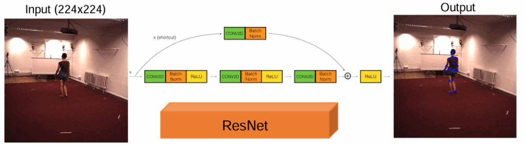
• We have fine-tuned different versions of the RN with the size (224 × 224) of input data to estimate the 2D human pose in the RGB image.
• We have fine-tuned the estimated model on the HU-3.6M-D, with 2D pose ground-truth determined based on 3D pose annotation data and the intrinsic parameters of the camera.
• We evaluate the estimated results based on the absolute estimated coordinates between the original data and the estimated data. From there, choose the best RN version with input data of 224 × 224 for 2D-HPE on the RGB image, and will have good results in 3D-

The paper is organized as follows. Section 1 introduces several backbones for detecting and estimating people on images. Section 2 presents the related studies on 2D-HPE methods. Section 3 presents the main idea and versions of RN. Section 4 shows and discusses the experimental results of 2D human pose estimation, and Section 5 concludes the paper and future works.

2. Related Works

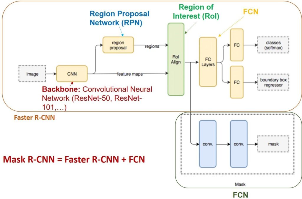
RN [14] is a backbone applied to many CNNs for feature extraction and object prediction in the first step such as Fast R-CNN [16], Faster R-CNN [17], Mask R-CNN [18], etc. Figure 1 shows the RN as the backbone in the Mask R-CNN network architecture. RN [14] is more efficient than other backbones like AlexNet [19], VGG [20], [21].

2D-HPE from RGB image data using CNN can be done by two methods [10]: regression methods, body part detection methods.

The regression methods use the CNNs model to learn joints location from the input ground-truth joints on the images to body joints or parameters of human body models/human skeleton to predict the key points on the human. In [22], the author proposed a Deep Neural Network (DNN) based on the cascade technique for regressing the location of body joints. The proposed CNN includes seven layers, the input image size of CNN is resized to 220 × 220 pixels. The cascade of pose regressors technique is applied to train the multi-layer prediction model. The first stage is the cascade starts with the initial position predicted over the entire input image. In the next stage, Deep Neural Net- works regressors are trained to predict a displacement of the joint locations with the correct locations in the previous stage. Thus, the currently predicted pose is refined based on each subsequent stage. In [23], a strategy of compositional pose regression based on the RN-50 [14]. The bones are parameterized and bone-based representation that contains human skeleton information and skeleton structure but did not use joint-based representation. The loss function is calculated based on each part of the human body, the joints are defined based on a constant origin point in the image coordinate system J₀. Each bone has a directed vector pointing from it to its parent. In [24], it is proposed a regression method that used two Soft-argmax functions (Block-A and Block-B) for 2D human pose estimation from images, Block-A provides refined features and Block-B pro- vides skeleton-part and active context maps. Two blocks are used to build one prediction block. Block-A used a residual separable convolution, the input feature maps are transformed into part-based detection maps and context maps by Block-B.

As for the body-part detection methods, a body-part detector is trained to predict the locations of human joints. In [13], it is proposed the stacked hourglass architecture for the training model to predict the positions of body joints on the heatmap in which the 2D annotation is used to generate the heatmap by 2D Gaussian heatmap method. The stacked hourglass repeats the bottom-up and top-down processing with intermediate supervision with the eight hourglasses. This CNN used the convolutional and max-pooling layers at a very low resolution and used then the top-down sequence of upsampling (the nearest neighbor upsampling of the lower resolution) and a combination of features across scales. The results of 2D-HPE on the MPII dataset based on the (PCKh@0.5) measurement are 90.9%, 99.0%, 97.0% are the results of the FLIC dataset on the (PCK@0.2) measurement.

In [25], it is proposed a two-branch CNN model, the body part detection is predicted from heatmaps by using the 2D keypoints annotation to generate the ground-truth confidence maps. The confidence maps are predicted by the first branch and the part affinity fields are predicted by the second branch. The part affinity fields are a novel feature representation of both location and orientation in- formation across the limb’s active region.

Most of the above studies were evaluated on the COCO [26], MPII [27] datasets and evaluated on the Percentage of Correct Keypoints PCK − % measure. This measure is usually based on the estimated joint length with the root joint length, without taking into account the absolute estimates of the 2D keypoints (estimated absolute coordinates and ground-truth coordinates).

3. 2D-HPE Based on The RN and Its Variations

2D-HPE is an intermediate result to estimate 3D human posture according to the method: 2D to 3D lifting methods and model-based methods [10]. Therefore, the 2D-HPE results have a great influence on the 3D-HPE results. The RN is applied in many studies on human pose estimation and

gives good results [28]-[29]. That is the motivation for us to carry out this study to select a model with good 2D pose estimation results. We compared results from different versions of the RN (RN-10, RN-18, RN-34, RN-50, RN-101, RN-152) [14] to select the best results.

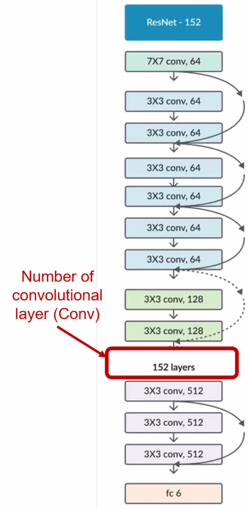
Residual Network (ResNet/RN) was introduced in 2015 and the 1st place in the 2015 ILSVRC challenge with an error rate is only 3.57%. Currently, there are many variations of RN architecture with a different number of layers. The named RN is followed by a number indicating the RN architecture with a certain number of layers. The RN have the number with each version RN-10 (10 Conv layers), RN-18 (18 Conv layers), RN-34 (34 Conv layers), RN-50 (50 Conv layers), RN-101 (101 Conv layers) ), RN-152 (152 Conv layers), as shown in Fig. 3.

RN is a DNN designed to work with hundreds or thou- sands of convolutional layers. When building a CNN net- work with many convolutional layers, the Vanishing Gradient phenomenon occurs, leading to bad model training results. The Vanishing Gradient phenomenon is presented as follows: The training process in DNN often uses Backpropagation Algorithm [30]. The main idea of this algorithm is that the output of the current layer is the input of the next layer and computes the corresponding cost function gradient for each parameter (weight) of the network. The Gradient Descent is then used to update those parameters.

The above process will be repeated until the parameters of the network are converged. Normally we would have a hyper-parameter (the number of epochs – the number of times the training set is traversed once and the weights updated) that defines the number of iterations to perform this process. If the number of loops is too small, then the network may not give good results, and vice versa, the training time will be longer if the number of loops is too large. However, in practice Gradients will often have smaller values at lower layers. As a result, the updates performed by Gradients Descent do not change much of the weights of those layers and make them not converged and the network does not work well. This phenomenon is called “Vanishing Gradients”. RN proposed to use a uniform “identity short- cut connection” connection to traverse one or more layers, illustrated in Fig. 4.

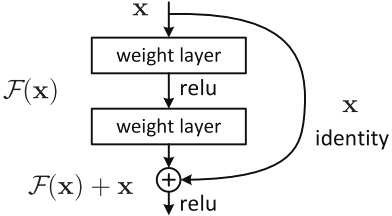
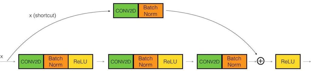
RN is like other CNNs, includes convolution, pooling, activation, and fully-connected layer. In RN, there appears a curved arrow starting at the beginning and ending at the end of the residual block as Fig. 4. In other words, it will add an input x value to the output of the layer, which will counteract the zero derivatives, since x is still added. With Hx being the predicted value, Fx is the label, the desired output Hx to be equal to or approximately Fx.

When the input of the network is the same as the output of the network, RN uses identity block, otherwise use the convolutional block, as presented Fig. 5.

In this paper, RN is a backbone for 2D-HPE and feature extraction. Recently, RN version 2 (v2) [14] is an improved version of RN version 1 (v1) for classification performance. The residual block [31] of RN v2 has two changes: A stack of 1×1-3×3-1×1 at the steps BN, ReLU, Conv2D is used; the Batch normalization and ReLU activation that comes before 2D convolution. Figure 6 shows the difference between RN v1 and RN v2.

4. Experimental Results

4.1. Dataset

To fine-tune, generate and evaluate the model and the estimated model, we use the benchmark HU-3.6M-D [32]. HU-3.6M-D is the indoor dataset for the evaluation of 3D- HPE from single-view of the cameras or multi-view of the cameras(the data is collected in a Lab environment from 4 different perspectives). This dataset is captured from 11 subjects/people (6 males and 5 females), the people perform with six types of action (upper body directions movement, full body upright variations, walking variations, variations while seated on a chair, sitting on the floor, various movements) which includes 16 daily activities (directions, discussion, greeting, posing, purchases, taking photo, waiting, walking, walking dog, walking pair, eating, phone talk, sitting, smoking, sitting down, miscellaneous). The frames are captured from TOF (Time-of-Flight) cameras, the data frame rate of the cameras is from 25 to 50 Hz. This dataset contains about 3.6 million images (1,464,216 frames for training – 5 people (2 female and 3 male), 646,180 frames for validation – 2 people (1 female and 1 male), 1,467,684 frames for testing – 4 people (2 female and 2 male)), 3.6 million 3D human pose annotations captured by the marker- based MoCap system. 3D human pose annotation of HU-3.6M-D consists of 17 key points arranged in order as shown in Fig. 7.

3D human pose annotations of HU-3.6M-D are annotated based on the Mocap system. The coordinate system of this data is the R-WCS. To evaluate the estimation results, we convert this data to the Camera Coordinate System (CCS). We based on the parameter set of the cameras and the formula for converting data from 2D to 3D of Nicolas [33] by Eq. 1.

where f x, fy, cx and cy are the intrinsics of the depth camera. P 3D_c is the coordinate of the keypoint in the CCS. Before evaluating the results of the 2D posture estimation, we re-projected the 3D human pose annotation from the R-WCS to the CCS using Eq. 2.

where R and T are the rotation and translation parameters to transform from the R-WCS to the CCS. P 3D_w is the coordinate of the keypoint in the R-WCS. We also projected to 2D human pose annotation using Eq. 3.

where P 2D is the coordinate of the keypoint in the image.

The source code and HU-3.6M-D have 2D annotation data as shown in link 1.

The authors have divided the HU-3.6M-D into 3 proto- cols to train and test the estimation models. Protocol #1 includes Subject #1, Subject #5, Subject #6, and Subject #7 for the training model, and Subject #9 and Subject #11 for the testing model. Protocol #2 is divided similarly to Proto- col #1. However, the predictions are further post-processed by a rigid transformation before comparing to the ground- truth. Protocol #3 includes Subject #1, Subject #5, Subject #6, Subject #7, and Subject #9 for the training model, and Subject #11 for the testing model. This dataset is saved in path 2.

4.2. Implementation

The input data of our network includes color/RGB image data and 2D human pose annotation. All images are resized to (224 × 224) before being fed to the network.

In this paper, the loss function for training the estimation model includes two parts: L₁, L₂. We used the loss function L₁ and Adam optimizer for the training process. First, we initialized the loss function L₁ for 2D coordinates predicted from RN. Then, we computed the loss function L₂ from the predicted 2D data. The loss function L of the whole training process is calculated as Eq. 4.

We set α and β to 0.1 to bring the 2D error (in pixels) into a similar range. The mean error was used to calculate the loss functions. We trained each network for 10 epochs, with the batch size being 32, Adam optimizer with the learning rate being 0.001, the number of the worker being 4.

In this paper, we used a PC with GPU GTX 970, 4GB for fine-tuning, training, testing the RN and its variations. The source code of fine-tuning, training, testing and development process was developed in Python language (≥3.6 version) with the support of the OpenCV-Python, Py-torch/Torch (≥1.1 version), CUDA/cuDNN 11.2 libraries. In addition, the support of some other libraries is required such as Numpy, Scipy, Pillow, Cython, Matplotlib, Scikit- image, TensorFlow ≥ 1.3.0, Keras ≥ 2.0.8, H5py, Imgaug, IPython. The source code for fine-tuning, training, testing is shown in link 3.

4.3. Evaluation Measure

To evaluate 2D-HPE, we evaluate in two phases. The first is to evaluate 2D human pose estimation results based on Eq. 5. It is the average distance between the 2D keypoint of the 2D ground-truth and the estimated 2D keypoint when using the trained model based on RN, the distance is calculated as the L₂ error value on the test set in pixels.

where N and J are the numbers of frames and number of joints (J = 17) respectively, p˜_i and p_i are predicted and ground-truth coordinates of i^th joint of the hand, L2 is the Euclidean distance between two points.

4.4. Results and discussions

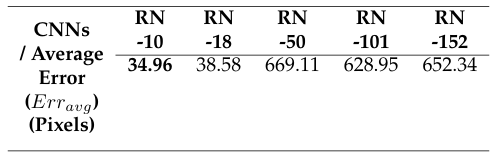
The pre-trained model of RN and its variants are shown in link 4. In this paper, we only evaluate the 2D-HPE on Protocol #1 and Protocol #3 of the HU-3.6M-D. The average error (Err_avg) between the 2D keypoint annotation and the estimated 2D keypoint of Protocol #1 of the HU-3.6M-D is shown in Tab. 1.

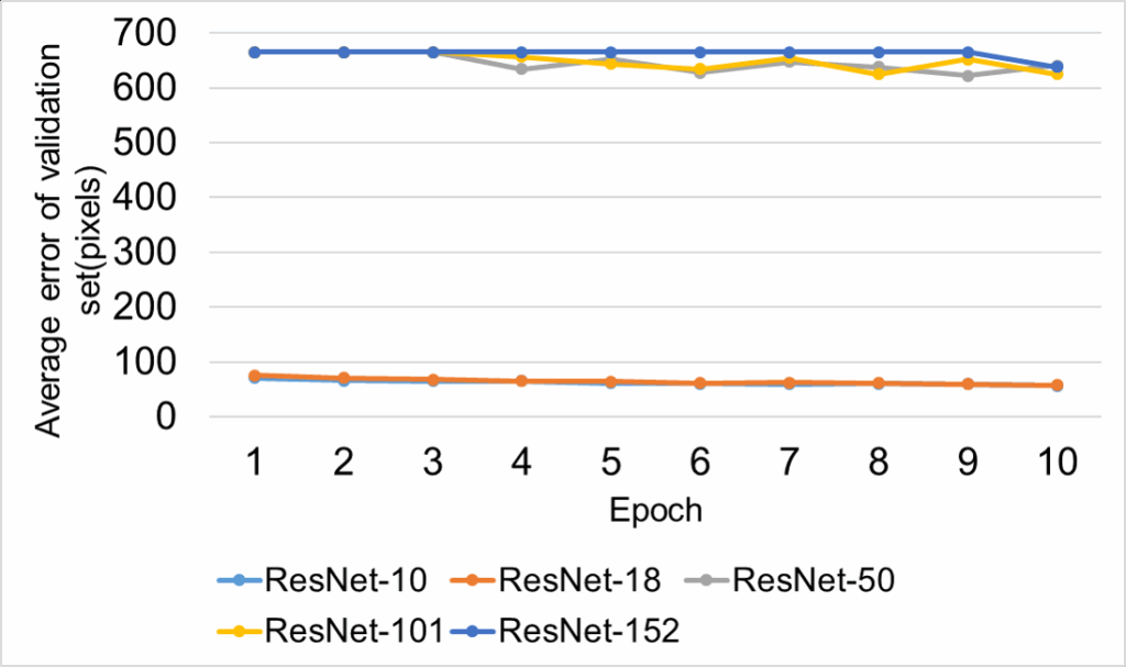
The average error (Err_avg) on the validation set following each epoch of Protocol #1 of the HU-3.6M-D is shown in Fig. 8.

In table 1, the average error of the RN-10 is 34.96 pixels, which is the best result on Protocol #1. The average error (Err_avg) between the 2D keypoint annotation and the estimated 2D keypoint of Protocol #3 of the HU-3.6M-D is shown in Tab. 2.

The average error (Err_avg) on the validation set following each epoch of Protocol #3 of the HU-3.6M-D is shown in Fig. 9

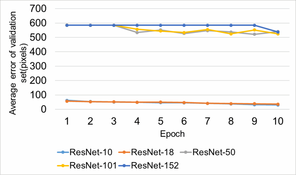
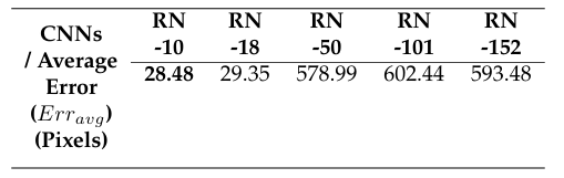
Table 1: The average error (Erravg ) (IP 1) between the 2D keypoint anno- tation and the estimated 2D keypoint of Protocol #1 of the HU-3.6M-D.

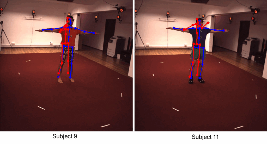
In table 2, the average error of the RN-10 is 28.48 pixels, which is the best result on Protocol #3. Figure 10 illustrates a 2D-HPE result on the image. The blue skeleton is the ground-truth of the human pose, the red skeleton is the estimated human pose. When we do the training RN-10 with 50 epochs, the average error (Err_avg) on the test set of Protocol #1 and Protocol #3 is 15.8 pixels, 12.4 pixels, respectively. Thus, increasing the number of training epochs reduces the estimation error.

In this paper, the RN-10 has better results than RN-18, RN-50, RN-101, RN-152 networks when training 10 epochs,

Table 2: The average error (Err_avg) between the 2D keypoint annotation and the estimated 2D keypoint of Protocol #3 of the HU-3.6M-D.

RN-10 network is a smaller CNN than other networks, which proves that a smaller number of convolutional layers will make the network converge faster. This is also consistent with the explanation that smaller networks will learn more efficiently than large CNNs [34].

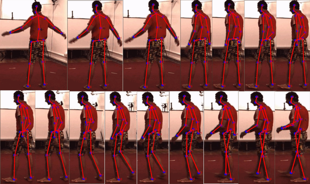
Figure 11 shows the result sequences of 2D-HPE of RN- 10 on Protocol #1 of Subject #9. The estimated 2D keypoints are blue-green nodes, the joints between the estimated 2D keypoints are the red lines.

5. Conclusions and Future Works

In this paper, we have performed a comparative study for 2D-HPE based on versions of RN (RN-10, RN-18, RN-50, RN-101, RN-152) on HU-3.6M-D with two evaluations Protocols (Protocol #1, Protocol #3). We have transformed 3D human pose annotation data to 2D human pose annotation. The average error of the RN-10 is 34.96 pixels, 28.48 pixels, respectively, which is the best result on Protocol #1, Proto- col #3. The results are evaluated and shown in detail and visually on the images. Therefore, RN-10 is a good CNN for estimating 2D human pose on images, this result can be used to estimate 3D human pose. In the future, we will use the human pose estimation results of RN-10 for 3D-HPE to compare with the studies of reference [35] and [9], which have the best results currently on the 3D-HPE.

Conflict of Interest: The paper is our research, not related to any organization or individual. It is part of a series of studies by 2D, 3D human pose estimation.

Acknowledgement: This research is funded by Tan Trao University in TuyenQuang, Viet Nam.

1. N. S. Willett, H. V. Shin, Z. Jin, W. Li, A. Finkelstein, “Pose2Pose: Pose Selection and Transfer for 2D Character Animation”, “Interna- tional Conference on Intelligent User Interfaces, Proceedings IUI”, pp. 88–99, 2020, doi:10.1145/3377325.3377505.
2. H. Zhang, C. Sciutto, M. Agrawala, K. Fatahalian, “Vid2Player: Con- trollable Video Sprites That Behave and Appear Like Professional Tennis Players”, ACM Transactions on Graphics, vol. 40, no. 3, pp. 1–16, 2021, doi:10.1145/3448978.
3. H. G. Weiming Chen , Zijie Jiang, X. Ni, “Fall Detection Based on Key Points of of human-skeleton using openpose”, Symmetry, 2020.
4. N. T. Thanh, L. V. Hung, P. T. Cong, “An Evaluation of Pose Estimation in Video of Traditional Martial Arts Presentation”, Journal of Research and Development on Information and Communication Technology, vol. 2019, no. 2, pp. 114–126, 2019, doi:10.32913/mic-ict-research.v2019.n2.864.
5. X. Zhou, Q. Huang, X. Sun, X. Xue, Y. Wei, “Towards 3d human pose estimation in the wild: A weakly-supervised approach”, “The IEEE International Conference on Computer Vision (ICCV)”, 2017.
6. G. Chandrasekaran, S. Periyasamy, K. Panjappagounder Rajaman- ickam, “Minimization of test time in system on chip using arti- ficial intelligence-based test scheduling techniques”, Neural Com- puting and Applications, vol. 32, no. 9, pp. 5303–5312, 2020, doi: 10.1007/s00521-019-04039-6.
7. G. Chandrasekaran, P. R. Karthikeyan, N. S. Kumar, V. Kumarasamy, “Test scheduling of System-on-Chip using Dragonfly and Ant Lion
   rnal of Intelligent and Fuzzy Systems,
   o. 3, pp. 4905–4917, 2021, doi:10.3233/JIFS-201691.
8. J. Martinez, R. Hossain, J. Romero, J. J. Little, “A Simple Yet Effective Baseline for 3d Human Pose Estimation”, “Proceedings of the IEEE International Conference on Computer Vision”, vol. 2017-Octob, pp. 2659–2668, 2017.
9. S. Li, L. Ke, K. Pratama, Y.-W. Tai, C.-K. Tang, K.-T. Cheng, “Cas- caded deep monocular 3d human pose estimation with evolutionary training data”, “The IEEE/CVF Conference on Computer Vision and Pattern Recognition (CVPR)”, 2020.
10. Q. Dang, J. Yin, B. Wang, W. Zheng, “Deep learning based 2D human pose estimation: A survey”, TPAMI, vol. 24, no. 6, pp. 663–676, 2021, doi:10.26599/TST.2018.9010100.
11. Z. Luo, Z. Wang, Y. Huang, L. Wang, T. Tan, E. Zhou, “Rethinking the Heatmap Regression for Bottom-up Human Pose Estimation”, “CVPR”, pp. 13259–13268, 2021, doi:10.1109/cvpr46437.2021.01306.
12. A. Bulat, G. Tzimiropoulos, “Human pose estimation via convolu- tional part heatmap regression”, “European Conference on Com- puter Vision”, vol. 9911 LNCS, pp. 717–732, 2016, doi:10.1007/ 978-3-319-46478-7_44.
13. A. Newell, K. Yang, J. Deng, “Stacked Hourglass Networks for Hu- man Pose Estimation”, “ECCV”, 2016.
14. K. He, X. Zhang, S. Ren, J. Sun, “Deep residual learning for im- age recognition”, “IEEE Conference on CVPR”, vol. 2016-Decem, pp. 770–778, 2016, doi:10.1109/CVPR.2016.90.
15. R. Zhang, L. Du, Q. Xiao, J. Liu, “Comparison of Backbones for Semantic Segmentation Network”, “Journal of Physics: Conference Series”, vol. 1544, 2020, doi:10.1088/1742-6596/1544/1/012196.
16. R. Girshick, “Fast R-CNN”, “Proceedings of the IEEE International Conference on Computer Vision”, vol. 2015 Inter, pp. 1440–1448, 2015, doi:10.1109/ICCV.2015.169.
17. S. Ren, K. He, R. Girshick, J. Sun, “Faster R-CNN: Towards Real-Time Object Detection with Region Proposal Networks”, IEEE Transactions on Pattern Analysis and Machine Intelligence, vol. 39, no. 6, pp. 1137– 1149, 2017, doi:10.1109/TPAMI.2016.2577031.
18. K. He, G. Gkioxari, P. Dollar, R. Girshick, “Mask R-CNN”, “ICCV”, 2017.
19. A. Krizhevsky, I. Sutskever, G. E. Hinton, “Imagenet classification with deep convolutional neural networks”, F. Pereira, C. J. C. Burges,
    L. Bottou, K. Q. Weinberger, eds., “Advances in Neural Information Processing Systems”, vol. 25, Curran Associates, Inc., 2012.
20. M. Lin, Q. Chen, S. Yan, “Network in network”, “2nd International Conference on Learning Representations, ICLR 2014 – Conference Track Proceedings”, pp. 1–10, 2014.
21. K. Simonyan, A. Zisserman, “Very deep convolutional networks for large-scale image recognition”, Y. Bengio, Y. LeCun, eds., “3rd Inter- national Conference on Learning Representations, ICLR 2015, San Diego, CA, USA, May 7-9, 2015, Conference Track Proceedings”, 2015.
22. A. Toshev, C. Szegedy, “DeepPose: Human Pose Estimation via Deep Neural Networks”, “IEEE Conference on CVPR”, 2014.
23. S. Liang, X. Sun, Y. Wei, “Compositional Human Pose Regression”, “ICCV”, vol. 176-177, pp. 1–8, 2017, doi:10.1016/j.cviu.2018.10.006.
24. D. C. Luvizon, H. Tabia, D. Picard, “Human pose regression by combining indirect part detection and contextual information”, Computers and Graphics (Pergamon), vol. 85, pp. 15–22, 2019, doi: 10.1016/j.cag.2019.09.002.
25. Z. Cao, T. Simon, S. E. Wei, Y. Sheikh, “Realtime multi-person 2D pose estimation using part affinity fields”, “IEEE Conference on CVPR”, vol. 2017-Janua, pp. 1302–1310, 2017, doi:10.1109/CVPR.2017.143.
26. T. Y. Lin, M. Maire, S. Belongie, J. Hays, P. Perona, D. Ramanan, P. Dol- lár, C. L. Zitnick, “Microsoft COCO: Common objects in context”, “Lecture Notes in Computer Science (including subseries Lecture Notes in Artificial Intelligence and Lecture Notes in Bioinformatics)”, l. 8693 LNCS, pp. 740–755, 2014, doi:10.1007/978-3-319-10602-1_
    48.
27. M. Andriluka, L. Pishchulin, P. Gehler, B. Schiele, “2d human pose estimation: New benchmark and state of the art analysis”, “IEEE Conference on Computer Vision and Pattern Recognition (CVPR)”, 2014.
28. X. Xiao, W. Wan, “Human pose estimation via improved ResNet50”, “4th International Conference on Smart and Sustainable City (ICSSC 2017)”, vol. 148, pp. 148–162.
29. Y. Wang, T. Wang, “Cycle Fusion Network for Multi-Person Pose Es- timation”, Journal of Physics: Conference Series, vol. 1550, no. 3, 2020.
30. N. Benvenuto, F. Piazza, “On the Complex Backpropagation Algo- rithm”, IEEE Transactions on Signal Processing, vol. 40, no. 4, pp. 967– 969, 1992, doi:10.1109/78.127967.
31. N. V. Hieu, N. L. H. Hien, “Recognition of plant species using deep convolutional feature extraction”, International Journal on Emerging Technologies, vol. 11, no. 3, pp. 904–910, 2020.
32. C. Ionescu, D. Papava, V. Olaru, C. Sminchisescu, “Human3.6m: Large scale datasets and predictive methods for 3d human sensing in natural environments”, TPAMI, vol. 36, no. 7, pp. 1325–1339, 2014.
33. N. burrus, “Kinect calibration”, http://nicolas.burrus.name/ index.php/Research/KinectCalibration.
34. X. Zhang, X. Zhou, M. Lin, J. Sun, “ShuffleNet: An Extremely Effi- cient Convolutional Neural Network for Mobile Devices”, “CVPR”, pp. 6848–6856, 2018.
35. C. Zheng, S. Zhu, M. Mendieta, T. Yang, C. Chen, Z. Ding, “3d hu- man pose estimation with spatial and temporal transformers”, “Pro- s of the IEEE International Conference on Computer Vision
    CV)”, 2021.

Citations by Dimensions

Citations by PlumX

Crossref Citations

This paper is currently not cited.

No. of Downloads per Month

No. of Downloads per Country