In a dynamic and complex bearing operating environment, current auto-encoder-based deep models for fault diagnosis are having difficulties in adaptation, which usually leads to a decline in accuracy. Besides, the opaqueness of the decision process by such deep models might reduce the reliability of the diagnostic results, which is not conducive to the subsequent optimization of the model. In this work, an ensemble deep auto-encoder method is developed and tested for intelligent fault diagnosis. To mitigate the influence of the changing operating environment on the diagnostic accuracy of the model, a tuning algorithm is used to adaptively adjust the parameters of the model, and a hypersphere classification algorithm is used to separately train different types of fault data. The encoder components in the ensemble model are automatically updated based on the diagnostic accuracy of the base encoder model under different operating conditions. To improve the reliability of the diagnosis results, the power spectrum analysis and Layer-wise Relevance Propagation algorithm are combined to explain the diagnosis results. The model was validated on three public datasets and compared with individual encoder methods as well as other common fault diagnosis algorithms. The results confirm that the model proposed is flexible enough to cope with changes in operating conditions and has better diagnostic and generalizing capabilities.

1. Introduction

Rolling bearings, whose health status affects the state of the running equipment, is one of the most common parts in industrial machinery [1]. Traditional fault diagnostic methods based on signal processing usually require employees to have not only complete knowledge of relevant industries [2], but also the ability of signal process and analysis [3].

As an intelligent diagnosis method that can automatically learn feature representation, deep auto-encoder has received extensive attention from scholars because it can reduce the requirement for practitioners and improve the accuracy of fault diagnosis when used for fault diagnosis.

Deep auto-encoder models originally used for fault diagnosis were typically stacked from individual-based encoder models, such as sparse auto-encoders (SAE)[4], compression auto-encoders (CAE) [5], denoising auto-encoders (DAE) [6], or their variants [7-9]. This kind of model can give full play to its advantages and obtain excellent diagnostic results when dealing with relatively simple data and less noise impact. However, bearings usually work in complex and noisy environments, so those traditional models often fail to accurately diagnose the fault signals with multiple jamming signals collected in real production environments.

To deal with such complex fault signals, some researchers combined different auto-encoders. For example, DAE and CAE are put together to form a new deep auto-encoder [10], or the integration of the three basic models SAE, DAE and CAE with different weight [11]. Compared with individual encoder models, these models have higher diagnostic accuracy when handling fault signals with noises. However, bearings are always in a changing environment during actual operation, and the diagnostic accuracy of such models are unstable due to their static structures and parameters. Some researchers have used tuning algorithms, such as particle swarm optimization [12-15] and cuckoo optimization[16], to optimize parameters under different working conditions. The diagnostic performance of these optimized models under different working conditions has been improved to a certain extent. However, the changing operating environment for bearings may also produce other factors that are detrimental to the diagnostic capability of the model, such as the unbalanced distribution of fault data samples [17]. Therefore, how to accurately detect various fault signals in the changing operating environment is still a major challenge in the field of fault diagnosis.

In addition, although the deep auto-encoder can provide high precision diagnosis results, the diagnosis results may not be trusted by experts at some point due to the opacity of its decision process. Only when users understand the reasons behind the model’s diagnostic behavior, can they fully trust the model and make a reliable decision according to the model’s diagnostic results [18] . Besides, it is difficult to optimize and migrate the model because the information of its training and decision-making process is usually hard to be reserved. One way to interpret deep models is to introduce additional modules into the model [19,20] that can directly output the diagnostic reasons during the fault diagnosis process. However, this approach will make the model more complex and requires more training time and datasets [21]. Another way is to use the ex-post interpretation model, which is retrospective after the decision is made [22, 23]. As a post-hoc interpretation model designed for computer vision, Layer-wise Relevance Propagation (LRP) [24-27] has been used to interpret fault diagnosis results based on time-domain data and convolution network. However, many current deep models for fault diagnosis are trained and validated based on frequency-domain data. To the best of our knowledge, LRP has not been used for diagnostic models based on ensemble deep auto-encoder and frequency-domain data. 

Therefore, in this paper, we propose an ensemble deep auto-encoder model, ALEDA, to improve the accuracy of fault diagnosis models under various operating conditions and the confidence of diagnostic results. Firstly, based on the arithmetic optimization algorithm[28], the parameters of the encoder model are optimized, which realizes the adaptive adjustment of the model parameters under different working conditions. Secondly, based on the hypersphere algorithm[29, 30], each type of data is trained separately, which alleviates the problem of unbalanced distribution of fault data samples caused by heterogeneities of working conditions. Then, the encoders are combined according to the diagnostic accuracy of the basic models optimized in specific condition, which is helpful to enhance the adaptability in a changing environment. Finally, the diagnostic results of the model are explained by using power spectral analysis and Layer-wise Relevance Propagation algorithm. It not only improves the reliability of the diagnosis results, but also provides enlightenment for interpreting the diagnosis results of the fault diagnosis model based on the frequency domain data. The model is validated on three public datasets and compared with other state-of-the-art fault diagnosis algorithms. The results demonstrate that the proposed model can flexibly respond to changes in working environments and has better capabilities of diagnosis and generalization.

The rest of this paper is organized as follows. Section 2 briefly introduces the basic theory of related methods. Section 3 describes the proposed model in detail. Section 4 verifies the effectiveness of the proposed model on three datasets, and analyzes and discusses the experimental results. Finally, conclusions are given in Section 5.

2. Related work

2.1. Arithmetic Optimization Algorithm

Compared with those classic optimization algorithms, the Arithmetic Optimization Algorithm[28] (AOA) is a new type of optimization algorithm whose effectiveness has not been verified in fault diagnosis models. And it is a group-based meta-heuristic optimization algorithm mainly including two stages of exploration and exploitation. In the exploration stage, the multiplication and division search strategy are mainly used to explore the search range to find the best solution. In the exploitation stage, the addition and subtraction search strategy are mainly used to optimize the solutions obtained in the previous phase. The algorithm defines two coefficients, one is (Optimization Phase Control parameter), used to control the phase of the algorithm (1); the other is (Optimized speed control parameter), used to control the updating speed of particle position (2).

where 𝑖 is the current iteration.  represents the maximum number of iterations of AOA algorithm. indicates the  maximum value of which is set to 0.9. represent the minimum values of  which is set to 0.2. And 𝛽 defines the development precision over iterations, which is fixed at 0.5.

The number 𝑘1,𝑘2,𝑘3 is randomly selected between 0 and 1. If the algorithm enters the exploration stage. And if 𝑘2<0.5 , the position of the particle is updated according to (3), otherwise according to (4).

Where are used to limit the optimization range of  parameter,  is used to control the speed of position updates in the search phase, which is set to 0.5.

And when 𝑘1<OPC(𝑖𝑖), the algorithm enters the exploration stage. And if 𝑘3<0.5, the position of the particle is updated according to (5), otherwise (6).

2.2. Auto-encoder

2.2.1. Sparse Auto-encoder (SAE)

SAE is built by stacking several sparse auto-encoders, where each sparse auto-encoder consists of an encoder and a decoder. The encoder can convert the input into a feature representation, while the decoder can reconstruct the input. Suppose the training set is where K is the number of samples. The feature representation  and reconstruction  can be expressed as (7) and (8).

Where 𝑓(∙) is the activation function, and  are the weight matrix of the encoder and decoder respectively,  and  are the bias vectors.

For each sparse auto-encoder, the cost function is given in (9).

Where is the input of the encoder,  is reconstruction,  is the λ coefficient specified by the user, 𝛽  is the coefficient of the sparse penalty term, and 𝜌  is the sparse factor.

2.2.2. Denoising Auto-encoder (DAE)

The DAE is constructed by stacking several denoising auto-encoders that learn feature representations and reconstruct data in the same way as a SAE. Unlike SAE, during training, data with noises is fed into the DAE. The noise input and cost function of each denoising auto-encoder can be expressed as (10) and (11), and the meanings of parameters are the same as those of SAE.

2.2.3.  Compression Auto-encoder (CAE)

CAE is constructed by stacking several compression auto-encoders which can learn more robust feature representation by adding a compression penalty term to its cost function. For each compression auto-encoder, the cost function is given in (12) and (13), and the meanings of parameters are the same as those of SAE.

2.3. Dynamic Hypersphere Algorithm

The dynamic hypersphere algorithm[29] refers to the use of perceptron to construct a dynamic feature space for each type of health training data separately, and to construct a corresponding hypersphere on the feature space of each type of data for their aggregation. By continuously reducing the error of the classification results, and updating the parameters, the hypersphere can be updated dynamically so that as many similar points as possible are constrained in the smallest possible sphere. Each class of data corresponds to a hypersphere. The dynamic hypersphere algorithm can not only take advantage of the perceptron on non-linear problems, but also perform well on unbalanced data by training and optimizing each type of data separately. Suppose there are  types of data, and each type of data has (𝑖=1,2,⋯,𝑚𝑚) samples. The initial value of  (the center of the sphere 𝑖 ) can be obtained from (14) and  (the distance from the sample to the center of the sphere 𝑖 ) can be expressed as (15).

Where represents the feature representation of 𝑗  neurons in the last layer of the encoder for the  class of training data, in other words,  is a reduced dimensional representation of the input data of class 𝑖 .

The loss function 𝐿(𝜃)  is defined as (16).

Where  is the penalty coefficient of each sphere,  is the penalty coefficient between spheres, and  is the accelerated convergence coefficient that plays a role in controlling the degree of punishment for sample segmentation. And  is the radius of sphere 𝑖 , which should be greater than 0.

𝐷𝑖(17) represent the total distance from the sample to the center 𝑖, 𝐷𝑖(18) represents the total distance between the data that does not belongs to class 𝑖 and 𝐷𝑖,𝑗(19) the center 𝑖 , and (19) is the separation distance between sphere 𝑖 and sphere 𝑗.

Calculate the distance from the new sample point to the center of each hypersphere, and take the class in which the closest hypersphere is located as the class of the new sample point.

2.4.  Layer-wise Relevance Propagation (LRP)

As an anomaly interpretation technique, LRP can provide correlation between input signals and diagnosis results. The greater the contribution of input layer neurons to model diagnosis, the higher the correlation score obtained during back propagation. By visualizing the correlation scores, the input neurons that contribute significantly to the output results of the model can be highlighted. The transmission mechanism of LRP is as follows:

It is known that the correlation  of neuron 𝑗 at layer 𝑙+1  can be decomposed to all neurons at layer 1. The greater the contribution of neuron 𝑖 at layer 𝑙 to neuron 𝑗 at layer 𝑙+1 at the stage of fault diagnosis, the higher the correlation score can be divided. And  can be expressed as (20).

After the correlation of all neurons in layer 𝑙+1 is decomposed, the correlation can be obtained by summation of all correlations  obtained by neuron 𝑖  in layer 𝑙 , and its mathematical expression is given in (21).

Further, the correlation coefficient  can be obtained through ε−rule , and its specific mathematical expression is given in (22).

 can be understood as the contribution of layer 𝑙 neuron 𝑖  to layer 𝑙+1 neuron 𝑗 , where  is the weighted activation of layer 𝑙+1 neuron 𝑗 by neuron 𝑖 of layer 𝑙 , and  is the weighted activation of layer 𝑙+1 neuron 𝑗 by all neurons of layer 𝑙 .

3. The proposed ALEDA method for intelligent fault diagnosis

To address the difficulties faced by deep auto-encoder models in fault diagnosis, we proposed an ensemble deep auto-encoder model with AOA and LRP, named ALEDA, which integrates DAE, CAE and SAE. DAE is used to learn useful information from input signals with noises; CAE is used to learn more robust feature representations. SAE is used to reduce the risk of over-fitting and a dropout layer is append to each hidden layer to enhance the ability. The training process of ALEDA model mainly includes four parts: optimizing the base encoder models to the best performance, determining encoder components of the ensemble model, obtaining the classification results of the ensemble model, and interpreting diagnosis results.

3.1 Optimizing the base encoder models

To maximize the diagnostic accuracy of the ensemble model in the face of a new operating environment, it is necessary to adjust the diagnostic accuracy of each encoder component to the maximum. The process can be divided into the following steps:

1. Determine the parameters to be optimized and the optimization algorithm to be used.

Since the learning rate affects the convergence of the model, and the number of nodes in the hidden layer directly affects the structure of the model, we use them as parameters to be optimized.  To verify the effectiveness of the AOA algorithm in passing, we choose the AOA algorithm to automatically adjust the parameters of the model.

2.  Determine the optimization range of the parameters.

A suitable search range will speed up the algorithm optimization. In this paper, empirical formula of neural network nodes of hidden layer (23) and pyramid geometric rules (24) and (25) are used to limit the optimization range of nodes of the hidden layer.

where represents the maximum number of nodes of the  hidden layer,  represent the minimum number of nodes of hidden layers respectively, are the number of nodes in the input layer and output layer respectively.

3. Determine the objective function of the optimization algorithm.

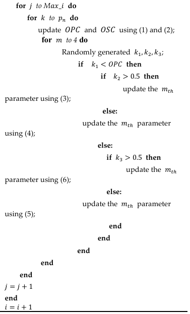
Since the goal of the optimization algorithm is to make the value of the loss function of the classifier as small as possible, it’s necessary to firstly determine the classifier. The hypersphere classifier can transform the same class of data into corresponding hyperspheres by training and optimizing each class of data separately, which alleviates the impact of data imbalance problems caused by changes in bearing operating conditions. Thus, the loss function of the hypersphere classifier (16) is used as the objective function of AOA. In addition, to take advantage of the encoder model while retaining the nonlinear advantage of the dynamic hypersphere algorithm, the encoder model is used instead of the original single-layer perceptron. The pseudo-code of parameter optimization algorithm for encoder network is given in Table 1.

3.2. Determining encoder components of the ensemble model

The next step is to design a strategy to combine the three encoders into an ensemble model so as to take full advantage of the three encoders to cope with the changing work environment. The strategies adopted in this paper are as follows:

Three auto-encoders  are selected to form the final ensemble model. First,  samples were randomly selected from the training set for dividing a new training set and the validation set by cross-validation. Next, SAE, DAE and CAE are used to learn the characteristics of the training set, and the hypersphere classifier is used to classify the training set, and the weights of the three basic encoders are updated according to (26). With each fold of cross-validation, the weight of each encoder changes dynamically. After the cross-validation, the encoder model with the highest weight is selected to compose the ensemble model, and it is trained with sample  for subsequent testing. The specific process is shown in Figure 1. The updating formula of weight  is given in (26), where the initial value is given in (27).

where 𝜌 is used to control the change degree of   is the verified accuracy.

3.3. Obtaining the classification results of the ensemble model

To get the diagnostic results of the ensemble model, the classification results of the three base encoder models need to be integrated. In this paper, Naive Bayes is used to further judge the classification results of the three classifiers to determine the final classification results. The specific process is given in Figure 2.

Table 1: The pseudo-code of the algorithm optimizing encoder parameters

It is assumed that there are  health conditions, and the total number of samples in the training set is and the sample number of each health condition is Firstly, the prior probability (28) of each type of sample is calculated and the Laplacian correction is made to it.

Next, after the training of each classifier is completed, their confusion matrix (Table 2) is calculated as the conditional probability (29).

Where  represents the number of samples actually labeled as  in the training set; and  represents the number of samples actually labeled as  but classified into  by the classifier.

Then, the posterior probability (30) of each health conditions of each classifier is obtained. For each test sample, the classification result of the classifier with the largest posterior probability is its final classification result.

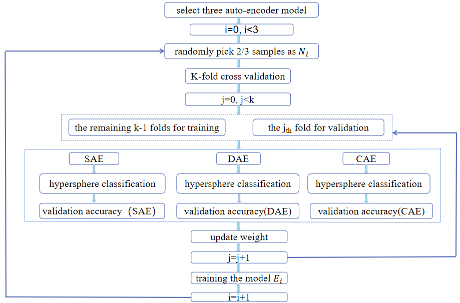
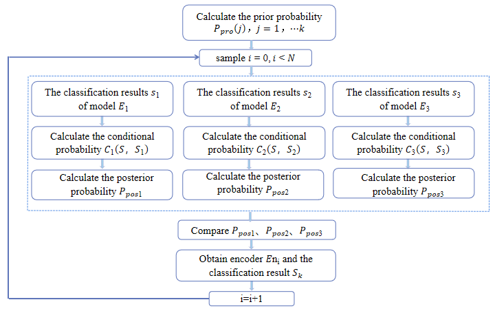
Table 2: The confusion matrix

3.4. Interpreting diagnosis results

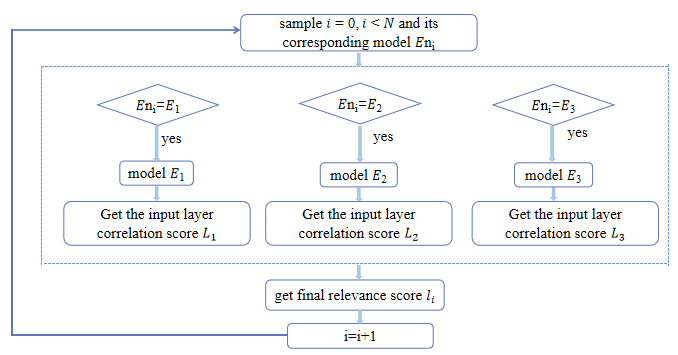
To interpret the diagnostic results, the correlation between the final combined classification results of each test sample and the input features needs to be obtained. First, it is necessary to know how much each neuron contributes to the results of each encoder model during the feature learning process of each hidden layer. Then, the correlation score between the classification results and the input features of each encoder model can be obtained. Next, the classifiers used in the previous stage are analyzed for each sample and the input layer correlation scores are recombined for each test sample. At last, the relationship between the diagnostic results of the ensemble model and the input features can be obtained. The specific process is given in Figure 3.

To more conveniently observe the prominent features of each test sample, the 100 neurons with the highest correlation score are visualized. Assuming a total of N test samples and neurons, is defined as the mean value of the correlation score of neurons in the input layer, and its mathematical expression is given in (31).

By counting the number of samples with correlation scores greater than in neuron 𝑗(𝑗 = 1,2,⋯,𝑚) at the input layer,  neurons with the greatest contribution to the final classification results of each sample can be obtained. 

3.5. Algorithm pseudo-code

Table 3: Pseudo-code of ALEDA algorithm

4. Experimental verification

4.1. Data Preprocessing

Since the discriminant information in the time domain signal is not easy to be recognized, and the frequency domain signal in each health condition has its own different statistical characteristic parameters, the original vibration signal is converted into frequency domain signal by fast Fourier transform for further analysis and judgment. Since the frequency domain coefficients of the original data are symmetric after FFT transformation, half of the frequency domain data is used as the input of the model.

4.2. Experimental Design

It is well-known that bearing usually works in noisy working environment. Therefore, due to the influence of external noise, the quality of the collected data will be reduced, which directly affects the diagnostic effect of the model[7]. It is true that an excellent model should have good anti-noise ability.  To evaluate the noise immunity performance of the model, the model was run separately in an additive White Gaussian noise (WGN) environment with different signal-to-noise ratios added. Besides, to reduce the influence of accidental factors on the experimental results, the average of five tests was taken as the result for each experiment.

We added WGN with SNR= 10dB, 5dB, -5dB and -10dB to the samples respectively to observe the influence of noise with different intensity on the sample (Figure 4). It can be observed that the frequency domain components of the original data are covered by noise after adding noise, especially when SNR = -10dB, the frequency component of the original signal is almost completely submerged and difficult to identify[7]. SNR is defined as (32).

where  is the signal power and  is the noise power.

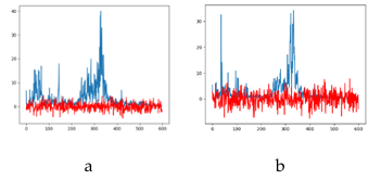
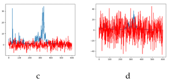
Figure 4: Power spectrum after adding noise (a) add 10dB noise (b) add 5dB noise (c) add -5dB noise (d) add -10dB noise

4.3. Evaluation indicators

Since multiple fault classes were considered in this paper, and the detection of each fault should be equally important, accuracy was selected as the main evaluation index. In addition, there may be data imbalance in the fault data, so precision and recall are used as evaluation indicators. The precision was used to judge the false positives of the model, and the recall rate was used to judge the false negatives of the model. Moreover, precision and recall restrict and influence each other, and F1 score takes both of them into consideration, so it was also taken as one of evaluation indicators. Their definitions are given in (33) – (36).

4.4. Validation on the Case Western Reserve University (CWRU) dataset

4.4.1 Data description

The motor bearing vibration data set of CWRU, as one of the widely used data sets, can be divided into ball fault, inner race fault and outer race fault according to different fault locations. Each fault location can be further divided into three categories: 7mils, 14mils and 21mils according to its severity. Thus, including healthy data, the data set can be divided into ten categories. The division of data sets is given in Table A1 in the Appendix. 

As the sampling frequency of the data is , and the motor speed changes between 1797 RPM and 1730 RPM, it can be calculated that the number n (37) of data points collected in each complete rotation of the rotating shaft is between 400 and 416. Therefore, to capture the impact of bearing failure at least once in each sample, the length of each sample is set to 1200 data points. For each category, it was divided into 400 samples based on the total number of data points. 80% of the samples were randomly selected as the training set and the rest as the test set. The original vibration signals are given in Figure A1 in the Appendix.

where  is the sampling frequency and  is the speed.

4.4.2 Model analysis

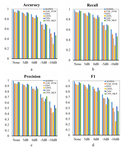
To verify that our strategy is effective in dealing with changing operating conditions, a series of comparative experiments were conducted. First, to verify the effectiveness of the AOA algorithm and the integration algorithm, the ALEDA model is compared with the manual parameter tuning model LEDA and the individual encoder models DAE, SAE, and CAE. Second, to verify the effectiveness of the strategy of dynamically selecting encoders based on weights, ALEDA was compared with the ensemble algorithm LEDA_Fix, where three encoders are fixed. Note that the classifiers used for comparison are all hypersphere classifiers.

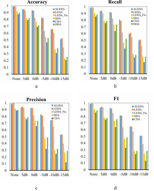
By observing the comparison of various evaluation indexes in Figure 5, it can be found that under various noise environments, the classification accuracy of ALEDA is almost equal to LEDA, and even slightly better than LEDA in some cases. This shows that the network parameters automatically selected by the AOA algorithm and the parameters selected by manual repeated experiments have the same effect in the fault diagnosis model. Secondly, by comparing LEDA and LEDA_Fix, it can be found that LEDA shows higher classification accuracy in all kinds of noisy environments. And the advantage of LEDA gradually expands with the increase of noise. In addition, by comparing with individual encoder model DAE, SAE and CAE, it can be found that the ensemble model has better performance in noisy environment. In summary, the parameter adjustment algorithm AOA and the integrated algorithm are beneficial to improve the efficiency of parameter adjustment and improve the classification accuracy of the fault diagnosis model.

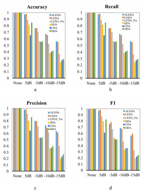
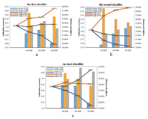
To understand the training process of our ensemble model when determining the composition of encoders, the weight changes process of the three encoders during the first experiment in a noise-free environment were recorded and analyzed (Figure 6). When the first encoder was selected (Figure 6 (a)), the initial weight of the three models were set to 33.33% and then the weights of the three encoders were updated according to Equation 26 after the first folding of cross-verification. The weight of SAE was increased to 33.65% due to its highest validation accuracy while the weight of CAE was reduced to 33.08% due to its lower validation accuracy than the other two models. In the second fold, the validation accuracy of CAE was still the lowest among the three, so its weight was again reduced to 32.96%, a decrease of 0.12%. And DAE and SAE are validated with the same accuracy, so the weight of each is increased by 0.06%.

In the third fold, the validation accuracy of SAE was still the highest, so its weight was further increased by 0. 06%. At the same time, DAE and CAE were reduced by 0. 03% respectively because of the same accuracy. In terms of overall performance, after the completion of cross-validation, SAE has the highest weight of 33.77%, which is better than the other two models, so it is determined as the final model. Figure 6(b) and Figure 6(c) show the changing process of the weight and verification accuracy when selecting the second and third encoders, respectively. Since the selection idea is the same as the above process, it will not be repeated here. At the end of training, an ensemble model consisting of SAE, DAE, and SAE can be obtained.

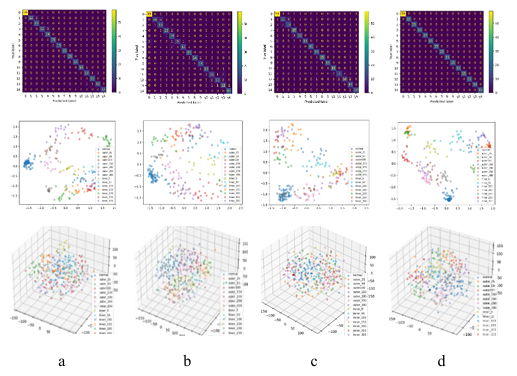
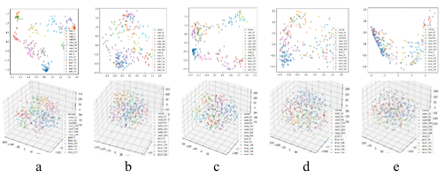
In addition, to intuitively compare the learning capability of feature representation between the ensemble model and the individual encoder model, the principal components of the ensemble model and each encoder model in a 5dB SNR environment were extracted using TSNE, and visualized as 2Ds and 3D plots. Meanwhile, the confusion matrix of each model is visualized. All these plots are placed in Figure 7, where each column is the same model.

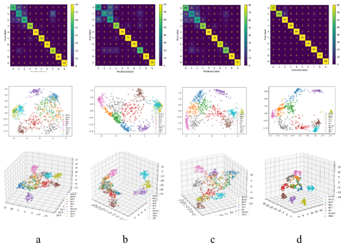
For the SAE model, only the outer race fault samples OR7 and OR21 with fault depths of 7mils and 21mils and the inner race fault sample IR21 with a fault depth of 21mils were significantly separated from the other samples. All other types of samples have different degrees of overlap, especially the ball fault samples with failure depths of 7mils, 14mils and 21mils, which have a larger amount of overlap. Therefore, only OR7, OR21 and IR21 were completely correctly classified, while a large number of samples in other categories were incorrectly classified. For DAE model, IR21 samples were completely separated from other samples, and there was a small amount of overlap between IR7 and IR14, IR7 and OR21, OR7 and OR21, and normal and B21. There was a large amount of overlap between the samples of other categories, so only IR21 was completely correctly classified, and some samples of other categories were incorrectly classified. Similarly, for CAE models, only IR21 samples were correctly classified. For ensemble model ALEDA, there was still a little overlap between the ball fault samples of the three fault depths, so a small number of samples were misclassified. However, compared with the three separate models, there was a significant improvement. Besides, there was a small amount of overlap between IR14 and B7, and a small amount of overlap between IR14 and OR14. Therefore, one IR14 sample was wrongly classified into B7, and one IR14 sample was misclassified into OR14. In general, ALEDA is superior to SAE, DAE and CAE in learning feature representation under 5dB SNR environment.

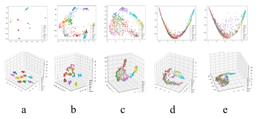
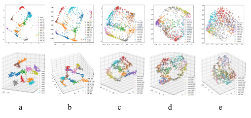
In addition, to observe the key features extracted by ALEDA under different noise levels, the principal components of the test samples in 5dB, 0dB, -5dB, -10dB and noise-free environment were extracted using TSNE, and visualized as 2Ds and 3D maps (Figure 8). It was found that in the noise-free environment, the test samples with different health status were separated obviously, and the different types of fault samples began to overlap gradually with the increase of noise.

4.4.3 Analysis of diagnostic results

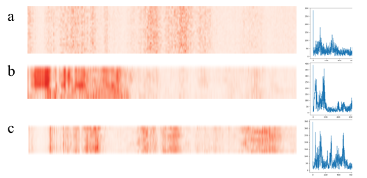
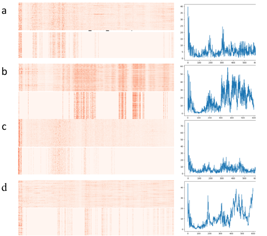
After obtaining the classification results of the ensemble model, the correlation scores of the input features can be obtained through the propagation mechanism of LRP. Correlation scores of the health test samples and the test samples with a fault depth of 21mils were visualized as heat maps where the higher the correlation scores, the higher the color saturation.

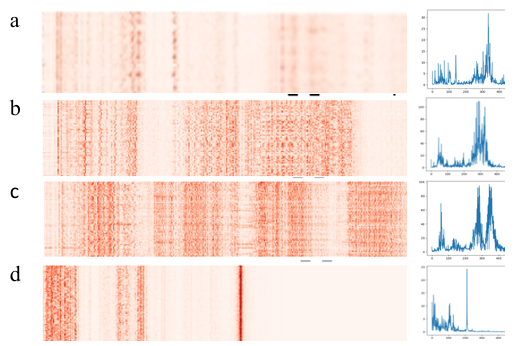
According to the heat map, the contribution of input features of each test sample to the diagnosis results can be obtained. And we can see that each type of fault has its unique salient characteristics. To find the relationship between these high-scoring input features and their corresponding fault categories, a few samples were drawn from each type of the testing data and their power spectrum were visualized. The heat and spectrum plots are placed in Figure 9, where each row is the same fault category.

In the traditional power spectrum analysis, when the peak value in the vibration spectrum is not equal to the multiple of the speed frequency, it means that the fault may occur. Further, if there are harmonics and side bands at the same time, the fault’s more likely to occur. In addition, the fault frequency varies due to different fault locations. That is, each failure happens on a particular frequency component. By comparing heat map and power spectrum, it can be seen that features with higher scores in the LRP heat map usually correspond to frequencies with larger amplitudes in the power spectrum map. Besides, the regions of high score aggregation in the heat map roughly correspond to the regions with dense side bands and harmonics in the power spectrum map. Therefore, we infer that features with high scores in the heat map are related to abnormal frequencies such as side bands and harmonics in the power spectrum map. Our model learns and classifies all kinds of fault data through the data points that are different from normal frequency.

4.4.4 Comparison with other intelligent diagnosis methods

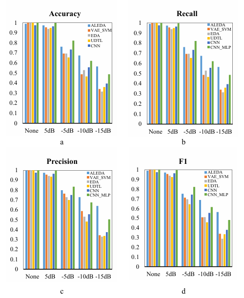
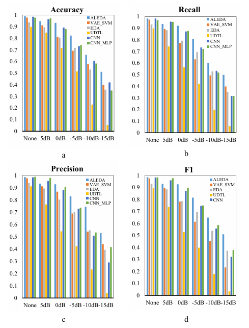
Compared with other intelligent fault diagnosis methods VAE_SVM (VAE for dimensional-reduction of data) [31], CNN_MLP [32], CNN, EDA(weighted integration) [33], UDTL (based on transfer learning)[34] . Five experiments were carried out for each algorithm in each noisy environment to get the average value where the parameters of the algorithm in this paper were tuned by the AOA algorithm in the first run, and the saved parameters were then directly called in other four experiments to improve the running efficiency of the algorithm.

accurately classify various faults in a noise-free environment, and both false negatives and false positives of each model perform well. With the increase of the noise in the data, the indicators of each model began to decline, but ALEDA performed better than VAE_SVM, EDA, UDTL and CNN. However, in 5dB and -5dB environments with little noise influence, all indexes of ALEDA are lower than CNN_MLP, which might be explained that CNN can extract deeper features for further classification by MLP with its powerful feature extraction ability. With the increase of noise, ALEDA gradually shows better classification ability than CNN_MLP.

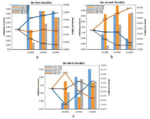
To explore the reason why ALEDA gradually outperforms CNN_MLP under high noise, the weight changes process of the three encoders during the first experiment in -10dB were recorded and analyzed (Figure 11). Compared with Figure 6, it can be found that SAE accounted for a large proportion in the ensemble model in the noiseless environment, while under -10dB noise environment, the DAE model exhibits better validation accuracy and stability during the selection of the first encoder (Figure 11(a)) and the second encoder (Figure 11(b)). When choosing the third encoder model (Figure 11(c)), the CAE model outperformed. It is obvious that the combined form of the DAE and CAE models further enhances the noise immunity of the ensemble model ALEDA.

4.5. Dataset of the American Association for Mechanical Failure Prevention Technology (MFPT)

4.5.1. Data description

MFPT bearing fault dataset can be divided into inner race fault and outer race fault according to different bearing fault locations, and each fault location can be further divided into 7 categories. Therefore, including healthy data, it is divided into 15 categories. Since the sampling rate of this data is 48,828sps and the input axis rate is 25Hz, about 1,953 data points can be collected every time when the axis is fully rotated. Therefore, to capture the impact of a bearing fault on each sample, the length of each sample was set to 2000 data points. The division of data sets and their load are given in Table A2 in the Appendix, and the original vibration signals are given in Figure A2 in the Appendix.  Finally, 80% of the samples were randomly selected as the training set and the rest as the test set. It is noteworthy that the number of healthy samples in the MFPT dataset is larger than the other faulty samples.

4.5.2. Model analysis

Like Section 4.4.2, ALEDA, LEDA, LEDA_Fix and DAE, SAE and CAE models of individual encoder were compared in various noise environments. As can be seen from Figure 12, the performance of ALEDA is like LEDA in various noise environments. And compared with LEDA_Fix, ALEDA and LEDA showed higher classification accuracy in various noise environments. ALEDA also achieved obvious advantages over individual encoder models SAE, DAE and CAE. Therefore, it can be concluded that by using the parameter tuning algorithms AOA, the ensemble algorithm and the hypersphere classifier the disgnostic accuracy is improved regardless of the operating environments.

T_SNE was used to extract the main components of the ensemble model and each encoder model in noiseless environment, and the two-dimensional visualization and three-dimensional visualization were carried out respectively. Meanwhile, the confusion matrix of each model was visualized. All these plots are placed in Figure 14, where each column describes the same model. By observing Figure 14, it can be found that in the three basic models, most of the samples of various health conditions cannot be completely separated, and there was sample overlap. While by ALEDA, most types of samples had clear boundaries that can be distinguished from other types of samples. In general, ALEDA is superior to SAE, DAE and CAE in learning feature representation. Figure 15 showed the main components of ALEDA at different noise levels.

4.5.3. Analysis of diagnostic results

Correlation scores and the power spectrum (Figure 16) of the fault test sample at 300 loads and the health sample were visualized. Due to the limited amount of data per category in the MFPT datasets, the heat map has a narrow width. Although the amount of data is small, each type of data shows its unique characteristics. By comparing the frequency spectrum diagram and the heat map, the location of the fault frequency component that affects each kind of data can be obtained, and fault diagnosis can be achieved by learning these key features.

4.5.4. Comparison with other intelligent diagnosis methods

The model ALEDA and several other fault diagnosis methods VAE_SVM, CNN_MLP, CNN, EDA and UDTL were respectively run in each noise environment and compared. As can be seen from Figure 17, the performance of ALEDA is similar to CNN_MLP and CNN in a noise-free environment. However, in a low-noise environment, say 5dB, both models based on convolutional neural network were slightly better than ALEDA. With the increase of noise, ALEDA gradually showed better classification ability. We’ve discussed the reasons in Section 4.4.4. In addition, ALEDA was always superior to VAE_SVM, EDA and UDTL in various noise environments.

4.6. Dataset of Jiang Nan University (JNU)

4.6.1. Data description

The JNU data set contains inner race fault, outer race fault, ball fault and normal data at speeds of 600, 800, and 1000 [35]. As the fault frequency of the same fault location changes with the change of rotation speed, the data set is divided into 12 types according to the fault location and rotation speed, and the division of the dataset is given in Table A3 in the Appendix. The original vibration signals are given in Figure A3 in the Appendix.

4.6.2. Model analysis

We compared ALEDA, LEDA, LEDA_Fix and DEA, SAE, CAE models in different noise environments (Figure 18). Overall, ALEDA showed better performance at all noise levels, proving that it has some advantages under different operating conditions.

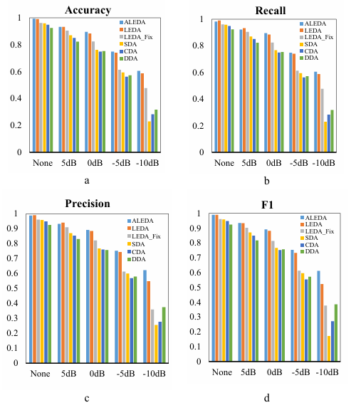
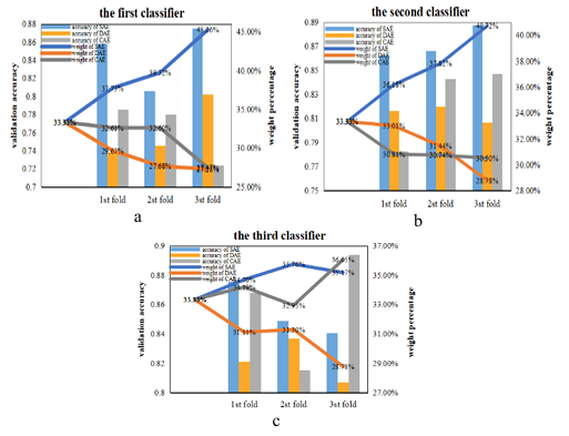
Figure 19 shows the weight changes process of the three encoders during training in the first experiment without noise. When the first encoder was selected (Figure 19 (a)), the initial weight of the three models were set to 33.33%. And in the triple fold of cross-validation, the validation accuracy of SAE has always been the highest, so its weight has been increasing. And at the end of the cross-validation, the weight of SAE (36.53%) was higher than that of the other two models, so it was identified as the final model. In the process of selecting the remaining two encoders, as shown in Figure 19(b) and Figure 19(c), SAE is still the one with the largest weight, so the composition of our final integration model is SAE, SAE and SAE.

Figure 20 show the main components and confusion matrix of ALEDA, SAE, DAE and CAE at 5dB SNR. For the basic models SAE, DAE and CAE, at 5dB SNR, the normal samples at 600 RPM were almost completely separated from other samples, and there was a large amount of overlap between the samples of other categories. As for the ensemble model ALEDA, although there is still a small amount of overlap between various samples, it has been greatly improved compared with the basic model.

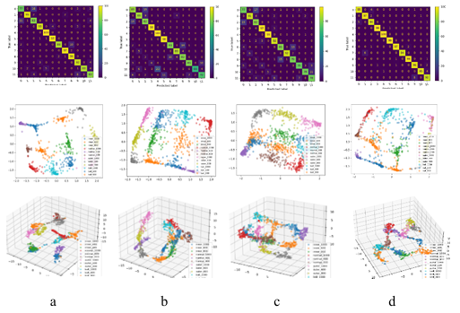
Figure 21 shows the main components of ALEDA at different noise levels. In the noise-free environment, the test samples with different health conditions were separated obviously. With the increase of noise, different types of fault samples began to overlap gradually.

4.6.3. Analysis of diagnostic results

Correlation scores of test samples at 1000 RPM were visualized as heat maps. Since the color difference between different features in the heat maps is not very large, the 100 features with the highest scores were visualized.  In addition, several samples were randomly selected from each type of fault and their power spectrum were visualized. All the images are placed in Figure 22. By observing the power spectrum and heat maps, it can be found that each type of fault has unique prominent features, and the features with high scores in the heat map can roughly correspond to the harmonic components in the power spectrum map. Therefore, it can be concluded that the features of high color saturation in the heat map are equivalent to the frequency of abnormal faults in the power spectrum map, and our model classifies the fault data by learning these features.  

4.6.4. Comparison with intelligent diagnosis methods

In this experiment, ALEDA and several other fault diagnosis methods, VAE_SVM, CNN_MLP, CNN, EDA and UDTL, were respectively run in SNR=5dB, 0dB, -5dB, -10dB and noiseless environment. And all running results were recorded in Figure 23. Through comparison, it is found that the performance of ALEDA was not much different from other models in the environment with little noise influence. With the reduction of SNR, ALEDA was gradually superior to other models. See section 4.4 for the reason.

5. Conclusions

In this paper, a new ensemble interpretable deep auto-encoder (ALEDA) method is proposed for intelligent fault diagnosis of rolling bearings. This method addresses the problem of diagnostic accuracy degradation of fault diagnosis models under variable operating conditions from three perspectives: adaptive adjustment of model parameters, targeted training of different types of fault data, and adaptive construction of integrated models. Power spectrum analysis and Layer-wise Relevance Propagation algorithm are combined to interpret the diagnostic results made by the model based on frequency domain data, which not only improves the reliability of the diagnostic results, but also provides enlightenment for interpreting the results. In addition, it is worth mentioning that this method verifies the effectiveness of the arithmetic optimization algorithm in the fault diagnosis model to a certain extent.

ALEDA was validated on three public datasets, including the CWRU, MFPT, and JNU. By comparing the ALEDA model with the manual parameter tuning model, the effectiveness of the arithmetic optimization in the fault diagnosis model based on deep auto-encoder was verified. In addition, by visualizing and comparing the main features extracted by ALEDA and the individual encoder models, it was found that ALEDA can learn more critical features. Moreover, the impact of noise on the diagnostic accuracy of the ALEDA model was explored by visualizing the features extracted by ALEDA under different noises. What’s more, ALEDA was compared with other advanced intelligent fault diagnosis methods at different noise levels. Various experimental results show that ALEDA is flexible enough to respond to changes in operating conditions and has excellent capabilities of diagnosis and generialization.

At present, ALEDA is only the ensemble of three basic encoder models. In future work, we will replace the basic model with the encoder variant model to explore whether the model’s robustness and diagnostic accuracy can be further improved. Additionally, the data processing of the hypersphere classifier in the overlapping regions will be a meaningful study. 

Conflict of Interest

The authors declare no conflict of interest.

Acknowledgements

Funding was received from the National Natural Science Foundation of China (61871061), which is gratefully acknowledged.

1.  X. Wang,Y. Zi,Z. He, “Multiwavelet denoising with improved neighboring coefficients for application on rolling bearing fault diagnosis”,Mechanical Systems and Signal Processing, vol.25, no.1, pp.285-304,2011, doi:10.1016/j.ymssp.2010.03.010.
2.  Z. Wang,L. Jia,Y. Qin, “Adaptive diagnosis for rotating machineries using information geometrical kernel-ELM based on VMD-SVD”,Entropy, vol.20, no.1, p.73,2018, doi:10.3390/e20010073.
3.  J. Xie,Z. Li,Z. Zhou,S. Liu, “A novel bearing fault classification method based on XGBoost: The fusion of deep learning-based features and empirical features”,IEEE Transactions on Instrumentation and Measurement, vol.70, pp.1-9,2020, doi:10.1109/TIM.2020.3042315.
4.  W. Sun,S. Shao,R. Zhao,R. Yan,X. Zhang,X. Chen, “A sparse auto-encoder-based deep neural network approach for induction motor faults classification”,Measurement, vol.89, pp.171-178,2016, doi:10.1016/j.measurement.2016.04.007.
5. C. Shen,Y. Qi,J. Wang,G. Cai,Z. Zhu, “An automatic and robust features learning method for rotating machinery fault diagnosis based on contractive autoencoder”,Engineering Applications of Artificial Intelligence, vol.76, pp.170-184,2018, doi:10.1016/j.engappai.2018.09.010.
6. F. Xu,X. Shu,X. Zhang,B. Fan, “Automatic diagnosis of microgrid networks’ power device faults based on stacked denoising autoencoders and adaptive affinity propagation clustering”,Complexity, vol.2020,2020, doi:10.1155/2020/8509142.
7. Y. Zhang,X. Li,L. Gao,W. Chen,P. Li, “Ensemble deep contractive auto-encoders for intelligent fault diagnosis of machines under noisy environment”,Knowledge-Based Systems, vol.196, p.105764,2020, doi:10.1016/j.knosys.2020.105764.
8. S. Haidong,J. Hongkai,Z. Ke,W. Dongdong,L. Xingqiu, “A novel tracking deep wavelet auto-encoder method for intelligent fault diagnosis of electric locomotive bearings”,Mechanical Systems and Signal Processing, vol.110, pp.193-209,2018, doi:10.1016/j.ymssp.2018.03.011.
9. H. Shao,H. Jiang,Y. Lin,X. Li, “A novel method for intelligent fault diagnosis of rolling bearings using ensemble deep auto-encoders”,Mechanical Systems and Signal Processing, vol.102, pp.278-297,2018, doi:10.1016/j.ymssp.2017.09.026.
10. H. Shao,H. Jiang,F. Wang,H. Zhao, “An enhancement deep feature fusion method for rotating machinery fault diagnosis”,Knowledge-Based Systems, vol.119, pp.200-220,2017, doi:10.1016/j.knosys.2016.12.012.
11. Y. Zhang,X. Li,L. Gao,W. Chen,P. Li, “Intelligent fault diagnosis of rotating machinery using a new ensemble deep auto-encoder method”,Measurement, vol.151, p.107232,2020, doi:10.1016/j.measurement.2019.107232.
12. W. Deng,R. Yao,H. Zhao,X. Yang,G. Li, “A novel intelligent diagnosis method using optimal LS-SVM with improved PSO algorithm”,Soft Computing, vol.23, no.7, pp.2445-2462,2019, doi:10.1007/s00500-017-2940-9.
13. H. Chen,D. L. Fan,L. Fang,W. Huang,J. Huang,C. Cao,L. Yang,Y. He,L. Zeng, “Particle swarm optimization algorithm with mutation operator for particle filter noise reduction in mechanical fault diagnosis”,International journal of pattern recognition and artificial intelligence, vol.34, no.10, p.2058012,2020, doi:10.1142/S0218001420580124.
14. D. Lee,J. Ahn,B. Koh, “Fault detection of bearing systems through EEMD and optimization algorithm”,Sensors, vol.17, no.11, p.2477,2017, doi:10.3390/s17112477.
15. C. Lee,T. Le, “An Enhanced Binary Particle Swarm Optimization for Optimal Feature Selection in Bearing Fault Diagnosis of Electrical Machines”,IEEE Access, vol.9, pp.102671-102686,2021, doi:10.1109/ACCESS.2021.3098024.
16. W. Zhang,G. Han,J. Wang,Y. Liu, “A BP neural network prediction model based on dynamic cuckoo search optimization algorithm for industrial equipment fault prediction”,IEEE Access, vol.7, pp.11736-11746,2019, doi: 10.1109/ACCESS.2019.2892729.
17. H. Qu,Z. Qiu,X. Tang,M. Xiang,P. Wang, “Incorporating unsupervised learning into intrusion detection for wireless sensor networks with structural co-evolvability”,Applied Soft Computing, vol.71, pp.939-951,2018, doi:10.1016/j.asoc.2018.07.044.
18. M. T. Ribeiro,S. Singh,C. Guestrin, “” Why should i trust you?” Explaining the predictions of any classifier”,”Proceedings of the 22nd ACM SIGKDD international conference on knowledge discovery and data mining”, pp.1135-1144,2016, doi:10.1145/2939672.2939778.
19. A. Vaswani,N. Shazeer,N. Parmar,J. Uszkoreit,L. Jones,A. N. Gomez,A. Kaiser,I. Polosukhin, “Attention is all you need”,Advances in neural information processing systems, vol.30,2017.
20. X. Li,W. Zhang,Q. Ding, “Understanding and improving deep learning-based rolling bearing fault diagnosis with attention mechanism”,Signal processing, vol.161, pp.136-154,2019, doi:10.1016/j.sigpro.2019.03.019.
21. Y. Yang,V. Tresp,M. Wunderle,P. A. Fasching, “Explaining therapy predictions with layer-wise relevance propagation in neural networks”,”2018 IEEE International Conference on Healthcare Informatics (ICHI)”, pp.152-162,2018, doi:10.1109/ICHI.2018.00025.
22. B. Zhao,C. Cheng,G. Tu,Z. Peng,Q. He,G. Meng, “An interpretable denoising layer for neural networks based on reproducing kernel Hilbert space and its application in machine fault diagnosis”,Chinese Journal of Mechanical Engineering, vol.34, no.1, pp.1-11,2021, doi:10.1186/s10033-021-00564-5.
23. J. Grezmak,J. Zhang,P. Wang,K. A. Loparo,R. X. Gao, “Interpretable convolutional neural network through layer-wise relevance propagation for machine fault diagnosis”,IEEE Sensors Journal, vol.20, no.6, pp.3172-3181,2019, doi:10.1109/JSEN.2019.2958787.
24. A. Binder,S. Bach,G. Montavon,K. Müller,W. Samek, “Layer-wise relevance propagation for deep neural network architectures”, pp.913-922,2016, doi:10.1007/978-981-10-0557-2_87.
25. S. Bach,A. Binder,G. Montavon,F. Klauschen,K. Müller,W. Samek, “On pixel-wise explanations for non-linear classifier decisions by layer-wise relevance propagation”,PloS one, vol.10, no.7, p.e130140,2015, doi:10.1371/journal.pone.0130140.
26. A. Binder,G. Montavon,S. Lapuschkin,K. Müller,W. Samek, “Layer-wise relevance propagation for neural networks with local renormalization layers”,”International Conference on Artificial Neural Networks”, pp.63-71,2016, doi:10.1007/978-3-319-44781-0_8.
27. A. Rios,V. Gala,S. Mckeever, “Explaining Deep Learning Models for Structured Data using Layer-Wise Relevance Propagation”,arXiv preprint arXiv:2011.13429,2020, doi:10.48550/arXiv.2011.13429.
28. L. Abualigah,A. Diabat,S. Mirjalili,M. Abd Elaziz,A. H. Gandomi, “The arithmetic optimization algorithm”,Computer methods in applied mechanics and engineering, vol.376, p.113609,2021, doi:10.1016/j.cma.2020.113609.
29. M. Du,Q. Yu,L. Ruisen, “Hypersphere Algorithm for Classification on Dynamic Feature Space”,CEA, vol.56, no.22, p.6,2020, doi:10.3778/j.issn.1002-8331.1908-0352.
30. J. Zheng,H. Qu,Z. Li,L. Li,X. Tang, “An irrelevant attributes resistant approach to anomaly detection in high-dimensional space using a deep hypersphere structure”,Applied Soft Computing, vol.116, p.108301,2022, doi:10.1016/j.asoc.2021.108301.
31. J. An,S. Cho, “Variational autoencoder based anomaly detection using reconstruction probability”,Special Lecture on IE, vol.2, no.1, pp.1-18,2015.
32. Z. Zhao,Q. Zhang,X. Yu,C. Sun,S. Wang,R. Yan,X. Chen, “Unsupervised deep transfer learning for intelligent fault diagnosis: An open source and comparative study”,arXiv preprint arXiv:1912.12528,2019, doi:10.48550/arXiv.1912.12528.
33. Y. Zhang,X. Li,L. Gao,W. Chen,P. Li, “Intelligent fault diagnosis of rotating machinery using a new ensemble deep auto-encoder method”,Measurement, vol.151, p.107232,2020, doi:10.1016/j.measurement.2019.107232.
34. Z. Zhao,Q. Zhang,X. Yu,C. Sun,S. Wang,R. Yan,X. Chen, “Applications of unsupervised deep transfer learning to intelligent fault diagnosis: a survey and comparative study”,IEEE Transactions on Instrumentation and Measurement, vol.70, no.3525828, pp.1-28,2021, doi:10.1109/TIM.2021.3116309.
35. K. Li,X. Ping,H. Wang,P. Chen,Y. Cao, “Sequential fuzzy diagnosis method for motor roller bearing in variable operating conditions based on vibration analysis”,Sensors, vol.13, no.6, pp.8013-8041,2013, doi:10.3390/s130608013.

Citations by Dimensions

Citations by PlumX

Crossref Citations

No related articles were found.