The problem of acoustic monochromatic radiation by boundary with a traveling distribution of phases of normal vibrational velocities is considered. It is shown that when the spatial frequency of the traveling phase of normal velocities approaches the wave number in the medium, the energy transfer from boundary   into a “sliding” (with respect to the boundary) sound wave can resonantly increase to a value many times greater than the energy transfer from of the in-phase boundary, correspondingly, into the normal one (with respect to the boundary) sound wave at the same modules of amplitudes of vibrational velocities of boundary. In addition, the resonant energy transfer of the boundary into a “sliding” wave is the greater, the larger the wave dimensions of the radiating pattern on boundary. It is shown that when a similar traveling distribution of sound pressure (instead normal velocity) is specified at the boundary, there is no resonance. The influence of the curvature of the radiating boundary on the above phenomenon of resonant radiation was studied. It is shown that the resonant radiation of the boundary with given running phases of normal velocities generates a tangential (with respect to the boundary) constant in time radiation reaction force. It is shown that for the case of a linear chain of equidistant monopoles (or pulsing spheres separated from each other by medium) with a traveling phase (a traveling wave antenna) of their oscillatory velocities, the resonance does not appear.

1. Introduction

It is usually well-known that there is radiation (acoustical or electromagnetic monochromatic field in the far zone) at the spatial frequency h₀ < k₀ (k₀ -wave number in the medium) of sources, and at the spatial frequency h₀ < k₀ of sources radiation is absent or very small [1-7]. This is probably why the researchers did not consider this area in sufficient detail. Below, using several examples of very simple boundary value problems [8], it is shown that radiation power with an increase in the spatial frequency h₀ from h_{0 = 0} to h₀ > k₀ (immediately before radiation falling to zero at h₀ > k₀) can reach infinity when approaching h₀ to k₀ to . This means the phenomenon of resonance, which is of particular interest to any physicist, especially since we are talking about such an important physical quantity as the surface density of the radiated power. On the other hand, it is known that the traveling amplitude distribution of radiating elements (separated from each other by the medium) in traveling wave antennas does not lead to resonant radiation [9]. In addition, many highly educated researchers, without delving into details (on the basis of the hastily applied relationship between pressure and velocity through the impedance of the medium), are inclined to declare that there is no fundamental difference between boundary radiation with a given pressure and boundary radiation  with a given normal velocity. Thus the purpose of this work is to fill the above-mentioned small, but very common (as experience shows) gaps in understanding the process of wave radiation.

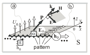
First, let’s consider a sound field excited in a compressible nonviscous linear medium (in a half-space ) by a traveling distribution (with a traveling phase [8])

of normal vibrational velocities on the surface S (plane surface S, z = 0,  r = (x,y,0 )), where U(w₀, h₀) is the complex amplitude of travelling wave on the time frequency w₀ and spatial frequency h₀ of normal vibrational velocities (Fig. 1-a). Below we will consider the radiation of various patterns (as modifications of (1)) with a traveling phase.

2. Plane (acoustical field)

Particle velocity v(x, z, t) and sound pressure p(x, z, t) are determined by potential ψ as

where  is the mass density of medium at z > 0.

Assuming the spatial two-dimensionality of the boundary value problem (i.e.), let us substitute the solution in the equation

( c is the speed of sound in a compressible medium) for the acoustic wave potential ψ(x, z, t) in the form

with functions X(x), Z(z), T(t), of separable variables x, z, t, in the absence of waves incident on the boundary z=0. In this case for wave potential ψ(x, z, t) (in the absence of incident waves and satisfying the boundary condition (1) or  we obtain the following expression

where

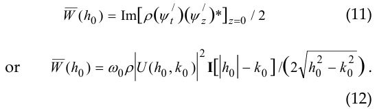
thus where  k_{0 =} ω₀/c .  Now we get the power flux density

at the boundary z = 0 . This is the work performed by a section of a strip of unit width (along the axis “x” ) and unit length (along the axis y) and averaged in time over a period 2π /ω₀ ). This is due to an abrupt change in the eigenvalue of the boundary value problem from purely real to purely imaginary when going from h₀ < k₀ to h₀ > k₀.  For the reactive power flow, we obtain the expression

of the energy transfer of the boundary z = 0 (into the half-space ) . P Lines (Pointing vector) of power flow go out of the plane z = 0  at an angle of inclination

However, when the traveling pressure

is set at the boundary z = 0, there is no resonance in the following corresponding  functions (instead (13), (14))

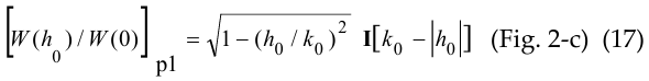
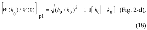
(contrary to superficial judgment about the relationship between pressure and velocity through the impedance of the medium, see Figs. 2-c, 2-d).

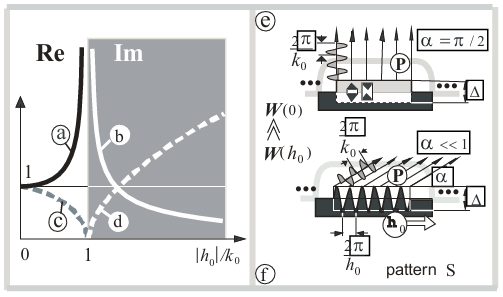
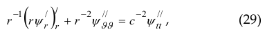
Below, the value [W(h₀) / W(0)]_n  (n = 1 – 5, i.e. in various modifications) will also be called the transmission function (in terms of power) of a spatial low-frequency filter (due to boundary value problem, Fig. 1) of spatial frequencies h₀ or also the normalized (by W(0) ) radiation resistance of a radiating pattern (pattern number n = 1 – 5 ) with spatial frequency h₀ along the vector called as phasor h₀ . Below the quantity U₀( x,t ) we also will call “pattern” with surface or boundary .   

The essence of the effect of resonant radiation: the wave generated by the pattern (1) at |k₀ – |h₀|| / k_{0 << 1}, takes much more energy for radiation (from the devices that support the pattern (1)) than the wave with h₀ = 0 (at the same fixed amplitude module ∆ = |U(h_{0, ω0)|} of pattern (1), Fig. 2-e, 2-f). In turn, devices that support pattern (1) must have an infinite internal impedance Z_u = ∞  (or not depend on any wave pressure at z > 0 ) or an impedance Z_u >> pc that is many times greater than the impedance pc of the medium (at ), for example: air (z > 0)—piezoceramic (thickness )—steel .

Here is another explanation of the effect. When |k₀ – |h₀|| / k_{0 < 1,} the solution of equation (3) in the half-space z > 0  is a plane sound wave with a wave potential , where A is the magnitude. To fulfill condition (1) at the boundary z = 0, the amplitude A of the radiated wave must be increased at  |h₀|→ k₀ (or  α→0 ) so that the projection of particle velocities in the radiated wave ψ onto the axis “z” coincides with pattern (1), which magnitude has been given independently on α. But supporting a given pattern (1) at α→0 requires more and more energy (energy of radiation).

3. Plane (electromagnetic waves).

The resonance characteristics (13), (14) described above are a property of the wave equation. Therefore, it is natural to assume the possibility of their appearance in the boundary value problem for an electromagnetic field. And indeed, for instance, the tangential electric field

( E₀ || (z = 0), h₀ || (z = 0) )  on the plane S or z = 0 (see Fig. 1-b) determines the electromagnetic field in the entire half-space  . When specifying a tangential electric field E₀ on the plane z = 0 (we emphasize, not an electric current or a source on the right side of the boundary conditions, namely the field E₀ ), we get the same resonance functions (13), (14) [ W (h₀) / W(0) ]₁ and .

4. Plane (acoustical radiation pressure).

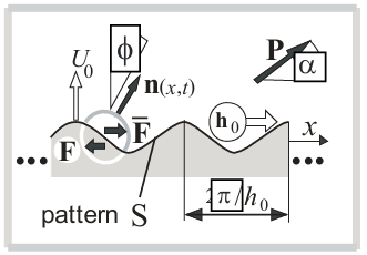
Let us return to the acoustic problem as in Section 2.  The pattern U₀ (x, t) creates a nonzero complex amplitude of  is the slope of the border z = 0 or a normal n (x, t), Fig. 3,   is equal to the following expression

Due to this, the local pressure force of the medium on the boundary z = 0 at the point x at t the moment has a tangential component

The average (for the time period and for the spatial period ) value of the force F (force per unit square of surface S,  z = 0 ) is equal to

where c_U = ω₀ / h₀ is the phase velocity of the pattern U₀ (x, t) (or the speed with which it would be necessary to translate the rigid profile

along the axis “x” in order to obtain the distribution U₀ (x, t) of normal velocities), W ( h₀ ) is the radiation power density of the boundary z = 0.

Obviously: is quadratic effect for U₀ (x, t) ; . On the other hand, the pattern acts on the liquid with a force that can generate a flow in  liquid. Thus, we have obtained the radiation reaction force for a perfectly linear compressible nonviscous medium (unlike [10]). Now consider the case when the pattern (1) of normal vibrational velocities (at the boundary z = 0 )

represented by a set of sinusoids at spatial frequencies { h_0n } and with amplitudes u_0n  ( n = 1,2,3,… ). Some of these sinusoids run to the left ( h_0n < 0 ), some of the sinusoids run to the right ( h_0n > 0 ). Accordingly, the projection ( < F >_x,t )_x of the tangential force < F >_x,t  (per unit area of ​​the plane z = 0 ) of the radiation reaction on the axis  “x”  is presented by term ( < F >_– )_x (caused by spatial harmonics running to the left, i.e. h_0n < 0 , n = 1,2,3,…  ) and term -( < F >₊ )_x (caused by spatial harmonics running to the right, i.e. h_0n  > 0 , n = 1,2,3,…  )

where, using (10) and (23), we can write

where I[ ξ ] -Heaviside step function (see (8)), . From (26)-(28) it is easy to see that the value (26) is the balance of the power of waves radiated to the right ( h_0n  > 0 ) and the power of waves radiated to the left ( h_0n < 0 ).

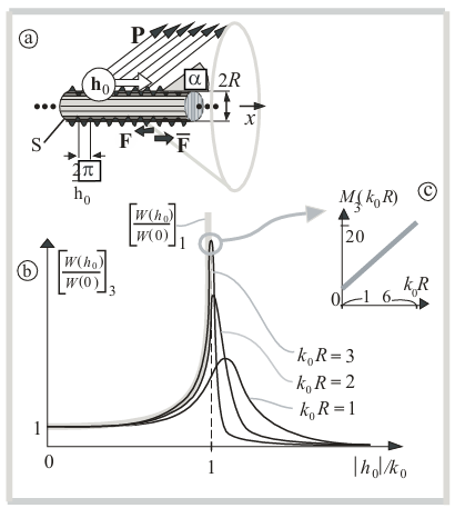
5. Cylinder (azimuthal phasor)

Next, we will continue to consider examples of resonant radiation by various patterns. Let’s consider patterns with a finite curvature of a bearing surface – an infinite cylindrical surface  of pattern with a cross-sectional radius R , on which a certain distribution U₀ (r, t) of normal vibrational velocities is given (Fig. 4-a).

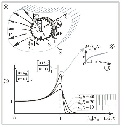
Using the cylindrical wave equation (instead (3))

(where r , ϑ are the corresponding cylindrical coordinates of point r) for pattern 

(the phase runs in the azimuthal direction ϑ, 0 ≤ ϑ < 2π, − ∞ < x < +∞ , ∂/∂x = 0 ) we obtain the normalized radiation resistance (Fig. 4-b)

of such a pattern, where, of course, only discrete points h₀ = n/R have a mathematical (and physical) meaning  ( H_n⁽²⁾ (ξ) is the Hankel function of the second kind of the n –th order, n = 1,2,3,… ). Looking at the evolution of the graphs of the magnitude [ W (h₀) / W(0) ]₂  with increasing k₀R , one could assume that

However, the convergence of these values ​​significantly slows down (this can be judged by the slowdown in the growth of the maximums (varying h₀ )

Power flux lines P exit the cylinder surface at an sliding angle α = across ( h₀/k₀ ) of inclination (i.e. cos(h₀p) = h₀/k₀, 0 ≤ α  ≤  π/2, see Fig. 4-c) and become straight radial in the far zone at the distance >> R²h₀. In book [4], for example, the author could get the resonance dependence (Fig. 2-a) if he would normalized the ordinate by (W₀) , and the abscissa by k₀ and considered the discrete azimuthal frequencies h₀ = n/R ( n = 1,2,3,… ) as interpolation nodes on the continuous axis of spatial frequencies.   Note that the integral flow of the Poynting vector P through an arbitrary closed cylindrical surface  (which embraces S ) is equal to the integral power flow on the surface  of the cylindrical radiating pattern (Fig. 4-a).

6.  Cylinder (axial phasor)

Now for the cylindrical wave equation (instead (29))

we consider the pattern (boundary condition)

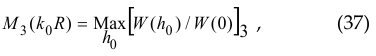
where the phase runs along the axis of the cylinder S ( − ∞ < x < +∞ , Fig. 5-a). So the normalized radiation resistance of such a pattern looks like

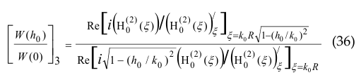
(Fig. 5-b). Note that here the argument  of the Hankel function H₀⁽²⁾ (ξ)  , when passing from |h₀|< k₀ to |h₀|> k₀ , turns from purely real to purely imaginary. The quantity [ W (h₀) / W(0) ]₃ is closing to [ W (h₀) / W(0) ]₁ faster than [ W (h₀) / W(0) ]₂  (see the function

varying h₀ , in Fig. 5-c). Power flux lines P exit the cylinder surface in a taper angle  α = across ( h₀/k₀ ) (i.e. cos(h₀p) = h₀/k₀, 0 ≤ α  ≤  π/2 , ).

7. Linear Chain of Acoustic Monopoles

Let us also consider the opposite example (with setting the speed, but without resonance) – a ruler (length 2L₀  ) 2N + 1 equidistantly (with a period of distributed pulsating spheres (acoustic monopoles) with radii (Fig. 6-a). Here, as in the previous sections, we set the normal vibrational velocity, but already on the surface of discrete pulsating spheres. The sinusoidal (with frequency ω₀ ) pulsations of the spheres are given the same amplitudes, and the phases of the pulsations are set linearly according to the law , where n is the sphere number is the phasor module h₀ . Thus this is a wellknown 3D travelling wave antenna [9]. Then, for the normalized radiation resistance of the pattern (chain of monopoles), we obtain the expression

where

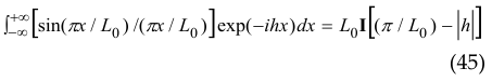
The function [ W (h₀) / W(0) ]₄  graph (Fig. 6-b) has no resonance, and

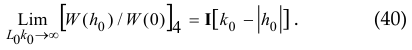
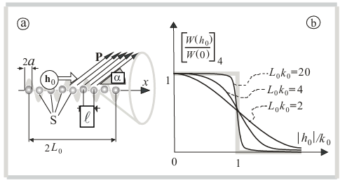
Figure 6. Linear chain of acoustic monopoles: (a) geometry of the boundary value problem; (b) normalized radiation resistance of the chain of monopoles at different wave sizes .

The difference between the boundary value problem and the previous ones lies in the absence of diffraction (small scattering on rigid fixed spheres) of the fields of pulsating spheres on each other due to their small wave sizes ( ka << 1 ) and relatively large distances between their centers. Surface  becomes lumped into a set of 2N + 1  small spheres (see Fig. 6-a). In other words, we summarize in the far zone the fields of the single pulsating spheres that each of them creates in a space free from other spheres. In the same way, there is no resonance when noninteracting spheres are placed on a ring (if we try to formulate the problem in Section 5 in a similar way). For it is indifferent (for [ W (h₀) / W(0) ]₄  ) to make given velocity or pressure on the spheres. This is probably the reason for the absence of resonance. The maximum radiation power of the line of monopoles corresponds to the direction of the Poynting vector P in a cone with an inclination angle α = across ( h₀/k₀ ) (i.e. cos(h₀p) = h₀/k₀, 0 ≤ α  ≤  π/2 , ). The radiation pressure is present as in above sections.

8. Spatially Localized Pattern on a Plane. 

For a rough estimate of the effect of amplification of acoustic radiation using a phasor h₀  ( at |h₀ | → k₀ ) at constant module of normal velocity amplitudes, we now consider (for the subsequent spectral representation) a pattern U₀( r, t ) = U₀( x, y, t ) localized on the plane z = 0 ( − ∞ < x, y < ∞ ) in the following form:

where -space scale of localization.   We need to estimate the ratio of the total power emitted by the pattern (41) at h₀ = 0 (Fig. 7–a) and the total power emitted by the pattern (41) at h₀ ≠ 0 (Fig. 7–b). Below we will consider the boundary-value problem of radiation as a low-frequency filter of spatial frequencies with a transmission coefficient (13) (in terms of power (Fig. 7-c)

where I [  ξ ]-Heaviside step function (see (8)), 

h_x, h_y are the components of the vector h ( h || ( z = 0))of the spatial frequency along the axes “x” and “y”, respectively (Fig. 7-d). Let’s write the spatial Fourier spectrum of pattern (41) as

Using the property

of the function Sin(ξ ) / ξ , we obtain Fourier spectrum

and,  accordingly, [ W (h₀) / W(0) ]_{5 = Q (h0) / Q(0)}, where

Fig. 7-e presents graphs of the magnitude [ W (h₀) / W(0) ]₅ for three wave sizes 2k₀L₀ of the pattern (41) and the dependence of the maximum (at varying h₀ ) value (as peak)

on wave size 2k₀L₀ (or area of spatial localization) of the pattern (41). It is not hard to see that for |k₀ -|h₀||/k₀ → 0 (i.e. |h₀| is closing to k₀ ) we obtain the value 

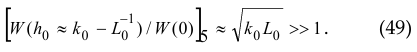
Figure 7.  On the spatially localized pattern (41) on the infinite plane: (a) “x” h₀ = 0  ; (b) “x” h₀ → K₀ ; (c)  one dimensional section [ W (h₀) / W(0) ]₁ of low pass filter of boundary problem for pattern (41); (d)  two dimensional view on the low pass filter characteristics (black area means the no radiation) of boundary problem for pattern (41); (e) normalized radiation resistance [ W (h₀) / W(0) ]₅ of pattern (41) at different wave sizes 2k₀L₀ , and value M₅ of its peak as function of wave dimension 2L₀k₀ of (41).

It can be seen from (49) that the larger the wave dimensions k₀L₀ of the pattern (41), the more effectively and resonantly the pattern with a running phase (at |k₀ – |h|| / k₀ <<1 ) radiates than the in-phase pattern (at h = 0 ) at a given fixed module U₀ ( 0, 0,0 ) of pattern amplitude.

Note that for finite wave sizes of the radiating pattern (sections 5-8, in contrast to sections 2-4), the real part W( h₀ )of field power flux on the surface of the pattern and the imaginary part  are nonzero at all spatial frequencies h₀.

9. Conclusion

In this work, the phenomenon of resonant sound emission by a boundary is analyzed analytically when a pattern is set on it in the form of a running sinusoidal spatial distribution of normal vibrational velocities at a certain temporal frequency (Section 1).

The initial problem is the resonant emission of sound by a spatially infinite harmonic distribution of normal velocities on an infinite plane (Section 2).

It is shown that setting a sinusoidal distribution of acoustic pressure on the plane does not generate resonant radiation (Section 2). In addition, it is shown that a linear chain of monopoles with a running phase of vibrational velocity amplitudes does not generate a radiation resonance (Section 7).

Further, the effect of the following factors on the magnitude of the resonant peak is estimated: surface curvature along the phasor (Section 5); surface curvature transversal to the phasor (Section 6); limitedness of the pattern in space (localization, Section 8).

A complete analogy of the phenomenon of resonant radiation in two problems is pointed out: (a) in the acoustic problem of Section 2;  in the problem of electromagnetic radiation of a flat boundary, on which a traveling distribution of a tangential electric field with a polarization parallel to the phasor is specified (Section 3).

In practice, if we need to obtain the highest radiation power of a certain pattern with a limited dynamic range of actuators, then it would be most expedient to excite a sliding (with respect to the pattern) wave with a distribution of normal vibrational velocities with a traveling phase, and not excite a normal (with respect to the pattern) wave with an in-phase distribution normal vibrational velocities.     

It has been shown that a resonantly radiating boundary with a traveling phase is capable of generating a time-constant tangential radiation reaction force and, consequently, can be used, for example, in designing an acoustic pump or for an active control of hydrodynamic boundary layer (Section 4).

Conflict of Interest

The author declares no conflict of interest.

Acknowledgements

This work was supported by the Russian Ministry for Science and Higher Education, Project No. 0030-2021-0009.

1. John William Strutt Rayleigh, The Theory of Sound; Volume 2, Franklin Classics, 978-0341849094, 2018.
2. L.D. Landau, E.M. Lifshitz, Course of theoretical physics (Fluid Me-chanics), Vol. 6, Butterworth-Heinemann, 2 edition, Jan 15, 1987.
3. L.M. Brekhovskih and O.A.Godin, Acoustics of Layered Media, Nauka, Moscow, 1989 (in Russian).
4. Eugen Skudrzyk, The Foundations of Acoustics (Basic Mathematics and Basic Acoustics), Springer, 1971.
5. James Lighthill, Waves in fluids, Cambridge University Press, Lon-don, New York, Melbourne, 1978.
6. Allan D. Pierce, Acoustics. An Introduction to Its Physical Principles and Applications, Third Edition, McGraw-Hill, Inc., 1980.
7. John D. Jackson, Classical electrodynamics, New York: Wiley, 1999.
8. V.V. Arabadzhi, Solutions to Problems of Controlling Long Waves with the Help of Micro-Structure Tools, Bentham Science Publishers, 2011.
9. C.H. Walter, Traveling Wave Antennas, McGraw-Hill, 1965, Dover, 1970, reprinted by Peninsula Publishing, Los Altos, California, 1990.
10. Robert T. Beyer, “Radiation pressure – the history of a mislabeled tensor,” Journal of Acoustical Society of America, vol. 63, no. 4, pp. 1025-1030, 1978, doi:10.1121/1.381833.

Citations by Dimensions

Citations by PlumX

Crossref Citations

This paper is currently not cited.