The derivation of the transfer function of the output filter of the electromagnetic compatibility of the inverter, loaded by RL-branch, proposed, which differs by taking into account the presence of resistances in the longitudinal and transverse branches of the L-shaped filter. The form of recording the voltage transfer function of an electrical transformer loaded by RL branch presented. A method for deriving the transfer function from the equations of the mathematical model of a single-phase two-winding transformer proposed. The transfer function derivation has made on T-shaped equivalent circuit of transformer basis, and takes into account the presence of resistance in the transformer windings, the winding connection group. To author’s opinion, results can be useful in the design of control systems and their mathematical models for electrical complexes, which include a sine-wave filter or a dv/dt filter and transformer.

1. Introduction

A sine-wave filter (SF) is one of the common options for the output filter of the electromagnetic compatibility (EMC) of an inverter with pulse-width modulation of voltage [1-4]. The SF performs the maximum approximation of the form of the output voltage of the inverter to a sinusoid, minimizing the value of the THDu, %. The task of the dv/dt filters is to reduce the rate of change of the pulsed voltage (smoothing, collapse of the pulse fronts) often to a level of less than 500 V/µs. In this case, the shape of the voltage on the load remains pulsed.

Electrical transformers [5-8] are very common and important elements in electrical systems and complexes, power management, automation. Even more common devices than EMC filters. An effective research tool in these areas is mathematical modeling, which requires the representation of data about an object in special formats. For example, to select the type of controller in an automatic control system, it is necessary to know the transfer function of the regulated object. The latter may include a transformer. Therefore, it is advisable to know the transfer function of the transformer.

The author could not find a record of transfer functions in the form of interest to him in publications, so he decided to derive them on his own.

2. Schematic Diagram of the L-Shaped Filter

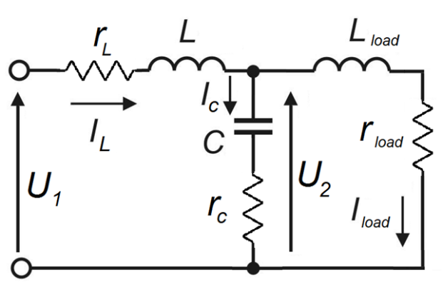
Each phase of an SF or dv/dt filter is an L-shaped filter with inductance L in the longitudinal branch and capacitance C in the transverse (see Figure 1). Strictly speaking, one should take into account the presence of the resistance of the inductive reactor in the longitudinal branch, including the resistance r_L in series with L . In the transverse branch, in series with C , in some cases, a damping resistor r_C is included. When used in an AC variable frequency drive, the SF or dv/dt filter is loaded on an active-inductive load, which can be represented by a series connection r_load and L_load.

3. L-Shaped Filter’s Transfer Function Derivation

To build control systems for electrical complexes containing an SF or dv/dt filter, you need to know the transfer function (TF) of the latter. Let us write down in the Laplace s-domain form the equations of the electrical circuit shown in the Fig. 1, using Kirchhoff’s laws.

$$i_L(s) = i_C(s) + i_{load}(s);\tag{1}$$

$$\qquad u_2(s) = i_C(s) \left( \frac{1}{C \cdot s} + r_C \right); \tag{2}$$

$$\qquad u_2(s) = i_{load}(s)(L_{load} \cdot s + r_{load});\tag{3}$$

$$\qquad i_L(s) = \frac{u_1(s) – u_2(s)}{L \cdot s + r_L}.\tag{4}$$

Express i_c(s) from equation (2):

$$i_C(s) = \frac{u_2(s)}{\frac{1}{C \cdot s} + r_C}.\tag{5}$$

Taking into account equation (5), we express from equation (1) i_L(s) , and from equation (3) we express i_load (s) :

$$i_L(s) = \frac{u_2(s)}{\frac{1}{C \cdot s} + r_C} + i_{load}(s);\tag{6}$$

$$\qquad i_{load}(s) = \frac{u_2(s)}{L_{load} \cdot s + r_{load}}.\tag{7}$$

Substituting equation (7) into (6), we obtain

$$i_L(s) = \frac{u_2(s)}{\frac{1}{C \cdot s} + r_C} + \frac{u_2(s)}{L_{load} \cdot s + r_{load}} = u_2(s) \left( \frac{1}{\frac{1}{C \cdot s} + r_C} + \frac{1}{L_{load} \cdot s + r_{load}} \right).\tag{8}$$

Let us equate the right parts of expressions (8) and (4), group the factors at the input and output voltages.

$$u_2(s) \left( \frac{1}{\frac{1}{C \cdot s} + r_C} + \frac{1}{L_{load} \cdot s + r_{load}} + \frac{1}{L \cdot s + r_L} \right) = u_1(s) \cdot \frac{1}{L \cdot s + r_L}.\tag{9}$$

Then we can write the filter’s TF by voltage as

$$H(s) = \frac{u_2(s)}{u_1(s)} = \frac{1}{\left( L \cdot s + r_L \right) \left( \frac{1}{\frac{1}{C \cdot s} + r_C} + \frac{1}{L_{load} \cdot s + r_{load}} \right) + 1}.\tag{10}$$

If we check, assuming r_C = r_L = L_load = 0  as in [9], then expression (10) will turn into the well-known equality (such a check can be performed at any stage of the transformation of the filter’s TF):

$$H(s) = \frac{1}{s^2 \cdot L \cdot C + \frac{L}{r_{load}} \cdot s + 1}.\tag{11}$$

Continuing the transformation of expression (10), we obtain a record of the TF, in which the parameters of the branches of the electrical circuit grouped in such a way that they can be denoted as time constants and resonant frequency:

$$H(s) = \frac{r_C C \frac{L_{load}}{r_{load}} \cdot s^2 + \left( \frac{L_{load}}{r_{load}} + r_C C \right) \cdot s + 1}{LC \frac{L_{load}}{r_{load}} \cdot s^3 + C \left[ L \left(1 + \frac{r_C}{r_{load}} \right) + \frac{L_{load}}{r_{load}} (r_L + r_C) \right] \cdot s^2 + \left[ \frac{L}{r_{load}} + \frac{L_{load}}{r_{load}} + C \left( r_L \left( 1 + \frac{r_C}{r_{load}} \right) + r_C \right) \right] \cdot s + \frac{r_L}{r_{load}} + 1} \\
= \frac{T_C \cdot T_{load} \cdot s^2 + (T_C + T_{load}) \cdot s + 1}{\frac{T_{load}}{\omega_0^2} \cdot s^3 + \left[ \frac{1}{\omega_0^2} \left( 1 + \frac{r_C}{r_{load}} \right) + T_{load}(T_C + r_L C) \right] \cdot s^2 + \left[ \frac{L}{r_{load}} + T_{load} + r_L C + T_C \left( \frac{r_L}{r_{load}} + 1 \right) \right] \cdot s + \frac{r_L}{r_{load}} + 1}.\tag{12}$$

If we accept r_C = r_L = 0 , and L_load  ≠ 0 , then expression (12) can be transformed in this particular case to the form

$$H(s) = \frac{\frac{L_{load} \cdot s + 1}{r_{load}}}{L \cdot C \cdot \frac{L_{load}}{r_{load}} \cdot s^3 + C \cdot L \cdot s^2 + \frac{L + L_{load}}{r_{load}} \cdot s + 1} = \frac{T_{load} \cdot s + 1}{\frac{T_{load}}{\omega_0^2} \cdot s^3 + \frac{s^2}{\omega_0^2} + \left( \frac{L}{r_{load}} + T_{load} \right) \cdot s + 1}.\tag{13}$$

In some cases, the value of r_L at r_C  ≠ 0 and L_load  ≠ 0 can be neglected, then expression (12) will take the form

$$H(s) = \frac{T_C \cdot T_{load} \cdot s^2 + \left( T_C + T_{load} \right) \cdot s + 1}
{\frac{T_{load}}{\omega_0^2} \cdot s^3 + \left( \frac{1}{\omega_0^2} + \frac{L}{r_{load}} T_C + T_C \cdot T_{load} \right) \cdot s^2 + \left( \frac{L}{r_{load}} + T_C + T_{load} \right) \cdot s + 1}\tag{14}$$

4. Transformer’s Transfer Function Derivation

For the synthesis of transformer’s TF, we take as a basis the equations of the mathematical model of a single-phase two-winding transformer [8], assuming that the conclusions obtained will be valid for each phase of multi-phase transformers.

$$\left\{ \begin{array}{l} v_1 – r i_1 – L_{\sigma 1} \frac{di_1}{dt} = v_{01}, \\[4pt] e_2 – r_2 i_2 = v_2 \end{array} \right. \tag{15}$$

where:

$$e_1 = -\left( v_{01} + L_{\sigma 1} \frac{di_1}{dt} \right); \tag{16}$$

$$\qquad e_2 = \pm \left( \frac{w_2}{w_1} v_{01} + L_{\sigma 2} \frac{di_2}{dt} \right). \tag{17}$$

EMF of the magnetizing branch of the primary winding v₀₁ :

$$v_{01} = L_m \left( \frac{di_1}{dt} + \frac{w_2}{w_1} \cdot \frac{di_2}{dt} \right) + r_m \left( i_1 + \frac{w_2}{w_1} \cdot i_2 \right) = L_m \frac{di_\mu}{dt} + r_m i_\mu. \tag{18}$$

On the right side of equation (17), for the I/I-0 connection group, select the “+” sign (consonant connection of inductances), and for I/I-6, the “–” sign (opposite connection). In expressions (16) – (18) the following designations are accepted: v and e  – voltage and EMF, V; i – current, A;  L_σ and L_m – leakage inductance of the winding and total inductance of the primary winding from the main magnetic flux, H; r and r_m – resistances of the winding and of the iron losses, Ohm; w is the number of winding turns. Indices 1 indicate belonging to the primary winding of the transformer, and indices 2 – to the secondary one; the  index at current means belonging to the magnetization branch of the T-shaped equivalent circuit (expression (18) is written for the case of r_m and L_m series connection). For the smallness of the active component of the magnetizing current of the transformer, we will take the assumption r_m = 0 for further transformations.

Let us rewrite system (15) taking into account (17) and (18) equations for the clock-notation group I/I-0:

$$\left\{ \begin{array}{l} v_1 – r i_1 – L_{\sigma 1} \frac{di_1}{dt} = L_m \left( \frac{di_1}{dt} + \frac{w_2}{w_1} \cdot \frac{di_2}{dt} \right); \\[8pt] \left( \frac{w_2}{w_1} L_m \left( \frac{di_1}{dt} + \frac{w_2}{w_1} \cdot \frac{di_2}{dt} \right) + L_{\sigma 2} \frac{di_2}{dt} \right) – r_2 i_2 = v_2 \end{array} \right.\tag{19}$$

To shorten the notation, we introduce the following designations:

$$L_1 = L_m + L_{\sigma 1};\tag{20}$$

$$\qquad L_2 = \frac{w_2^2}{w_1^2} \cdot L_m + L_{\sigma 2}.\tag{21}$$

Using (20) and (21) equations, we rewrite equation (19):

$$\left\{ \begin{array}{l} v_1 = r_1 i_1 + L_1 \frac{di_1}{dt} + \frac{w_2}{w_1} \cdot L_m \frac{di_2}{dt}, \\[6pt] 0 = r_2 i_2 – L_2 \frac{di_2}{dt} – \frac{w_2}{w_1} L_m \frac{di_1}{dt} + v_2 \end{array} \right.\tag{22}$$

We write equation (8) in the Laplace s-domain form

$$\left\{ \begin{array}{l} v_1(s) = r_1 i_1(s) + L_1 \cdot s \cdot i_1(s) + \frac{w_2}{w_1} \cdot L_m \cdot s \cdot i_2(s); \\[6pt] 0 = r_2 i_2(s) – L_2 \cdot s \cdot i_2(s) – \frac{w_2}{w_1} L_m \cdot s \cdot i_1(s) + v_2(s) \end{array} \right.\tag{23}$$

Let the load connected to the terminals of the secondary winding of the transformer, that is, to  v₂(p) voltage, be represented by a series connection of r_load and L_load. Then the current in the secondary winding can be expressed as 

$$i_2(s) = \frac{v_2(s)}{r_{load} + L_{load} \cdot s}.\tag{24}$$

Let us rewrite the second equation of system (23) taking into account (24)

$$0 = \left( \frac{r_2}{r_{load} + L_{load} \cdot s} – \frac{L_2 \cdot s}{r_{load} + L_{load} \cdot s} + 1 \right) \cdot v_2(s) – \frac{w_2}{w_1} L_m \cdot s \cdot i_1(s).\tag{25}$$

Let us express i₁(s) from the first equation of system (23) taking into account equation (24).

$$i_1(s) = \frac{v_1(s)}{r_1 + L_1 \cdot s} – \frac{\frac{w_2}{w_1} \cdot L_m \cdot s \cdot v_2(s)}{(r_1 + L_1 \cdot s)(r_{load} + L_{load} \cdot s)}.\tag{26}$$

Let us rewrite equation (25) taking into account equation (26) and perform some transformations:

$$
v_1(s) \cdot \frac{w_2}{w_1} \cdot L_m \cdot s \cdot (r_{load} + L_{load} \cdot s) = v_2(s) \cdot \Big\{
r_1 (r_{load} + r_2) \\
+ \left[ r_1 (L_{load} – L_2) + L_1 (r_{load} + r_2) \right] \cdot s \\
+ \left[ L_1 \cdot L_{load} – L_1 \cdot L_2 + \frac{w_2^2}{w_1^2} \cdot L_m^2 \right] \cdot s^2
\Big\} \tag {27}$$

We express from equation (27) the voltage TF of the transformer.

$$W(s) = \frac{v_2(s)}{v_1(s)} = \frac{\frac{w_2}{w_1} \cdot \frac{L_m \cdot r_{load}}{r_1 \cdot (r_{load} + r_2)} \cdot s \cdot \left(1 + \frac{L_{load} \cdot s}{r_{load}}\right)}{1 + \left( \frac{L_{load} – L_2}{r_{load} + r_2} + \frac{L_1}{r_1} \right) \cdot s + \left( \frac{L_1 \cdot (L_{load} – L_2) + \frac{w_2^2}{w_1^2} \cdot L_m^2}{r_1 \cdot (r_{load} + r_2)} \right) \cdot s^2} \tag {28}$$

We can write equation (28) in the form

$$W(s) = \frac{A \cdot s + A \cdot T_{load} \cdot s^2}{1 + B \cdot s + C \cdot s^2} = \frac{A \cdot s \cdot (1 + T_{load} \cdot s)}{1 + B \cdot s + C \cdot s^2}.\tag{29}$$

where is the load time constant

$$T_{load} = \frac{L_{load}}{r_{load}}.\tag{30}$$

For the I/I-0 connection group the difference in simulation results must be only as inverted phase of output voltage signal.

Let’s introduce a special multiplier  for right side of equation (28), which is responsible for belonging to one of the  winding connection groups in accordance with clock-notation rules. Let G = 1 , if I/I-0, and G = -1 , if I/I-6.

Now we can rewrite equation (29) in the form

$$W(s) = G \cdot \frac{A \cdot s + A \cdot T_{load} \cdot s^2}{1 + B \cdot s + C \cdot s^2}.\tag{30}$$

5. Simulation Results Discussing

Mathematical transformations derived for practical use is recommended to be justified with a simulation study. Because of this the author has constructed by means of OrCAD [10] computer models of L-shaped filter and single-phase transformer. Figure 2 demonstrates electric circuit-like (upper picture) and of block-diagram type (lower picture) variants of L-shaped filter models. The block-diagram type model based on equation (10). The electric circuit-like model based on Figure 1 scheme.

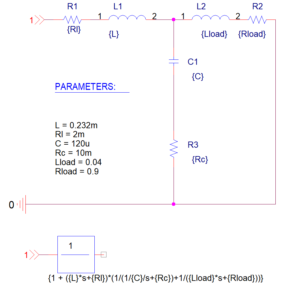
Figure 3 demonstrates simulated Bode diagram for both types of computer models of L-shaped filter with the same parameters: graphs are totally coincide.

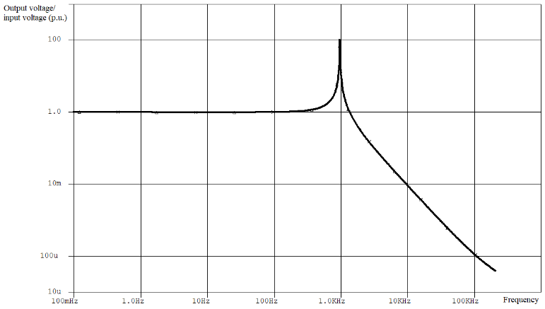
Figure 4 shows simulated response of the L-shaped filter computer models to the input voltage signal of the “step” type of 1.0 V amplitude. We can observe minor discrepancies in the graphs at the end of the transient process only. For ease of comparison, graph 1 in Figure 4 shown inverted.

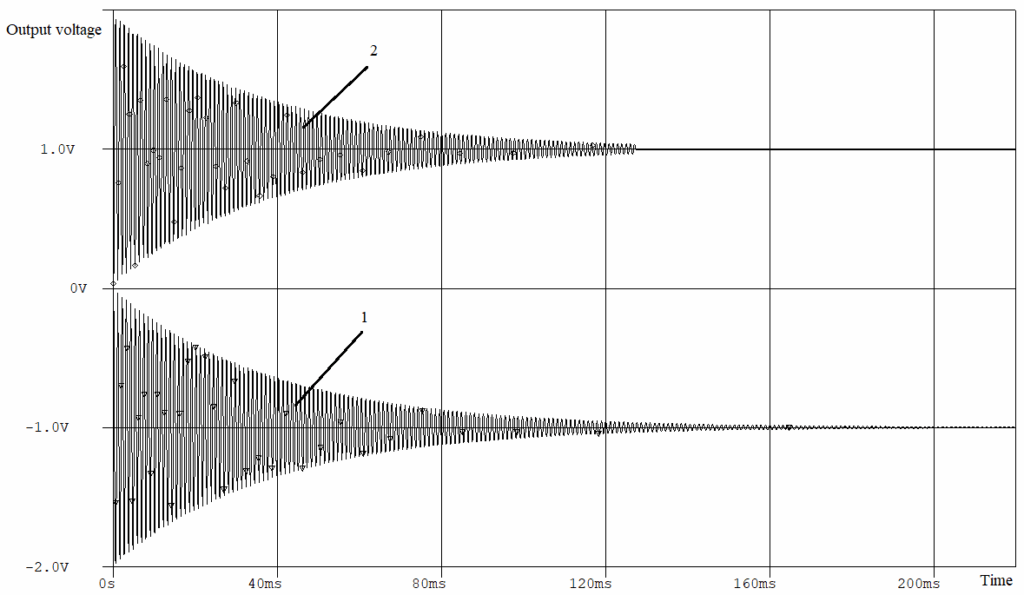
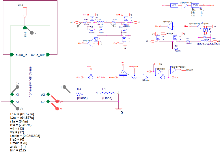
Figure 5 demonstrates the block-diagram type computer model of the single-phase transformer.

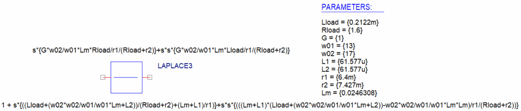
Figure 6 demonstrates the Electric circuit-like computer model of the single-phase transformer. This model designed in form of hierarchical block [8, 10].

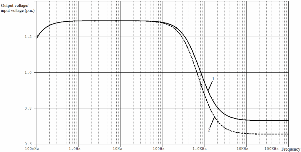
In Figure 7 we can see simulated Bode diagram for both types of computer models of the single-phase transformer (I/I-6 or I/I-0) with the same parameters: graphs are coincide at low and medium frequencies area, but there is a significant discrepancy at high frequency area.

Comparing the resulting Bode diagrams, we can assume that models of different types will work equally in the low and medium frequencies, but in the high frequency range, the waveforms will differ markedly. This is exactly what you can see in Figures 8 – 10.

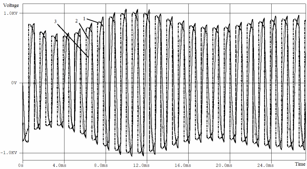
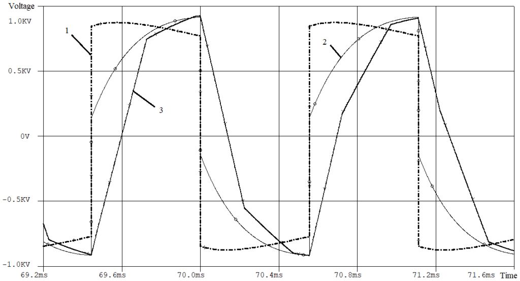
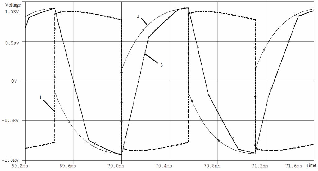
With a polyharmonic input voltage, the low-frequency shape of the output voltage envelope is treated the same by both models. Almost the same amplitude of the output voltage. But the shape of the output voltage for different models is different due to the presence of high-frequency components in the spectrum. Given the shape of input voltage 1, the shape of the output voltage graph 2 is more realistic.

6. Conclusion 

The derivation of the transfer function of the low pass L-shaped filter (for example output filter of the electromagnetic compatibility of the inverter), loaded by RL-branch, is proposed, which differs by taking into account the presence of resistances in the longitudinal and transverse branches of the L-shaped filter.

As a result of the mathematical transformations done, the transfer function of the transformer was obtained in a form suitable and convenient for practical use in the design of automatic control systems in which the control object (or its component) is an electric transformer. The transfer function is derived on the basis of the T-shaped equivalent circuit of the transformer, and takes into account the presence of resistance in the transformer windings, the winding connection group.

The adequacy of mathematical transformations for the derivation of transfer functions is confirmed by the results of computer simulation using OrCAD. As a result of the simulation, it was found that the response of the model based on the transfer function (block-diagram type) in the high-frequency region visibly differs from the response of the circuit model. This can lead to distortion of high-frequency signals and polyharmonic voltage shapes.

The achieved results can be useful in the design of control systems and their mathematical models for electrical complexes, which include a sine-wave filter or a dv/dt filter and electrical transformer.

1. B. Seunghoon, Choi Dongmin, Bu Hanyoung, Cho Younghoon, “Analysis and Design of a Sine Wave Filter for GaN-Based Low-Voltage Variable Frequency Drives,” Electronics, vol. 9 (345), pp. 76-89, 2020, doi:10.3390/electronics9020345.     
2. B. Anirudh Acharya, Vinod John, “Design of output dv/dt filter for motor drives,” 2010 5th International Conference on Industrial and Information Systems, 2010, doi: 10.1109/ICIINFS.2010.5578641.
3. M. Yu. Pustovetov, S.A. Voinash, “Analysis of dv/dt Filter Parameters Influence on its Characteristics. Filter Simulation Features,” 2019 International Conference on Industrial Engineering, Applications and Manufacturing (ICIEAM), pp. 1-8, 2019, doi:10.1109/ICIEAM.2019.8743007.
4. M. Pastura, S. Nuzzo, M. Kohler and D. Barater, “dv/dt Filtering Techniques for Electric Drives: Review and Challenges,” IECON 2019 – 45th Annual Conference of the IEEE Industrial Electronics Society, 2019, doi: 10.1109/IECON.2019.8926663.
5. Z. Aleem, S. L. Winberg, A. Iqbal, M. A. E Al-Hitmi and M. Hanif, “Single-Phase Transformer-based HF-Isolated Impedance Source Inverters with Voltage Clamping Techniques,” IEEE Transactions on Industrial Electronics, vol. 66, iss. 11, pp. 8434-8444, 2019, doi: 10.1109/TIE.2018.2889615.
6. A. Orlov, S. Volkov, A. Savelyev, I. Garipov and A. Ostashenkov, “Losses in three-phase transformers at load balancing,” Revista Espacios, vol. 38, no. 52, p. 37, 2017.  
7. V. Bosneaga, V. Suslov, “Investigation of Supply Phase Failure in Phase-Shifting Transformer with Hexagon Scheme and Regulating Autotransformer,” 2021 International Conference on Electromechanical and Energy Systems (SIELMEN), 2021, doi: 10.1109/SIELMEN53755.2021.9600358.  
8. M.Yu. Pustovetov, “A universal mathematical model of a three-phase transformer with a single magnetic core,” Russian Electrical Engineering, vol. 86, iss. 2, pp. 98-101, 2015, doi: 10.3103/S106837121502011X.
9. R.J. Pasterczyk; J.-M. Guichon, J.-L. Schanen and E. Atienza, “PWM Inverter Output Filter Cost to Losses Trade Off and Optimal Design,” 2008 Twenty-Third Annual IEEE Applied Power Electronics Conference and Exposition, 2008, doi: 10.1109/APEC.2008.4522764.     
10. J. Keown, OrCAD PSpice and Circuit Analysis, Upper Saddle River: Prentice Hall, 2001.

Citations by Dimensions

Citations by PlumX

Crossref Citations

This paper is currently not cited.

No. of Downloads per Month

No. of Downloads per Country