SiC ceramics are excellent materials applied at high temperatures because of their lightweight, excellent high-temperature strength, and high thermal shock resistance. For better engineering properties, we made SiC with fractal lattices. Stress-strain behavior and modulus changes from room temperature to 1,250 oC were analyzed using LAMMPS S/W, a molecular dynamics program. As a result of this study, it was confirmed that the modulus of elasticity of SiC crystals changed in the range of about 475 GPa to 425 GPa as it increased from room temperature to 1,250 oC. The stress-displacement characteristics of SiC crystals, which could not be measured at a high temperature of 1,000 oC or higher, could be ensured.

1. Introduction

A fractal is a geometric shape in which some small pieces are similar to the whole [1]. This characteristic is called self-similarity; in other words, a geometric structure with self-similarity is called a fractal structure. The word was first coined by Benoit Mandelbrot, and is derived from the Latin adjective fractus, meaning to be fragmented [2]–[3].

Fractal structures are found not only in natural objects but also in mathematical analysis, ecological calculations, and motion models appearing in topological space and are fundamental structures of nature [4]–[5]. You can even find rules that govern seemingly erratic and chaotic phenomena behind the scenes. The science of complexity is a science that studies the complexity of irregular nature that science has not understood so far and finds the hidden order therein. An order that can be expressed as a fractal appears in the chaos theory representing the science of complexity [6]–[7].

Fractal geometry is a branch of mathematics that studies the properties of fractals [8, 9]. This also applies to science, engineering, and computer art. Fractal structures, such as clouds, mountains, lightning, turbulence, shorelines and tree branches, are frequently found in nature. Fractals are of- ten used for practical purposes and can be used to represent very irregular objects in the real world. Fractal techniques are used in many fields of science and technology in image compression [10]–[11]. Fractals found in nature are easy to find.

1.1. Fractal Example (Nature)

1.1.1. Lightning

Lightning discharges in the same way as a staircase over and over again. Since the route is complicated by various conditions such as humidity, atmospheric pressure, and temperature, it has a meandering shape rather than a straight line. Although it looks irregular, the overall shape and each branch form a similar structure. That is, it has a fractal structure of self-similarity [12, 13].

1.1.2. River Stream

The part and the whole of the river resemble each other. The appearance of the Nile and the Han River are similar overall, and the appearance of the river in any region has a similar shape. The appearance of the tributaries and the river as a whole is similar. Much rain creates many junctions in the mountains. Each of these becomes a small river, and the act of meeting a large stream and extending into a small stream is repeated [14, 15].

1.1.3. Tree

When a tree is divided into a large branch, various branches are formed, and several small branches are also divided from this small branch. Each tree has its own fractal dimension. The fractal shape of these trees serves to evenly distribute the transport of water and nutrients throughout the tree [16, 17].

1.1.4. Coral

As colonies grow outward through agglomeration, the material is continuously deposited on the outwardly growing surface. It has a fractal dimension in principle similar to that of a tree root [18]–[19].

1.1.5. Clouds

A very uniform fractal, about 1.35 dimensions for cumulus clouds. A cloud created by a random condensation process takes on the form of a fractal as the generated water droplets attract the surrounding water droplets [20, 21].

1.1.6. Romanesco Broccoli

When grown, Romanesco broccoli develops a thorn-like appearance, with one part of the thorn showing the same self-similarity to the whole [22, 23].

1.1.7. Lizard sole

If you zoom in on the lizard’s sole, the surface of the sole has a fractal structure, which increases friction [24].

1.1.8. Bismuth

Element number 83 is self-similar in the pattern of atomic arrangement, and fractal structures can be easily found in outer space [25, 26].

1.1.9. Lung

The blood vessels in the lungs have a fractal structure and are said to be the most efficient for oxygen exchange [27, 28].

1.2. Fractal Examples (Structures)

Fractals can be easily found even in the patterns of high- strength structures.

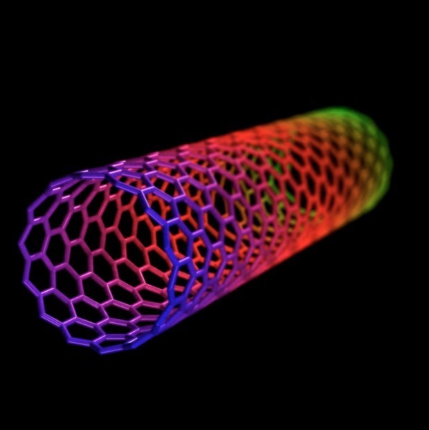
1.2.1. Carbon nanotube

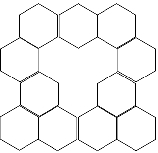
It is in the form of a tube by repeating the hexagonal shape. It has very high strength and shows self-similarity.

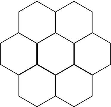
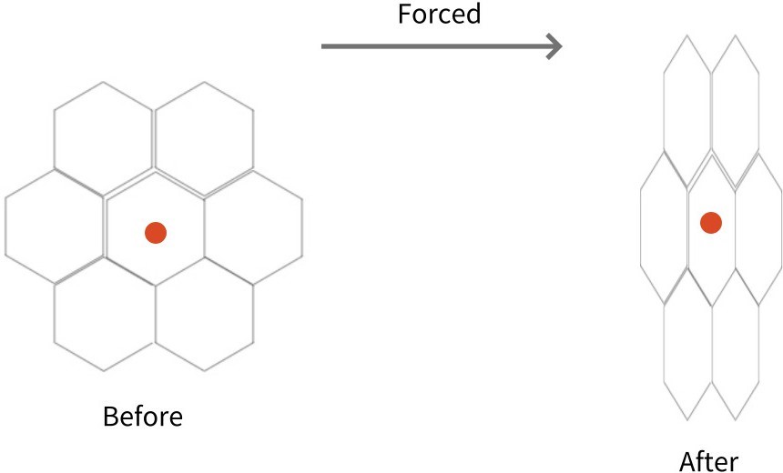
1.2.2. Honeycomb

The honeycomb repeats the hexagonal shape to show self- similarity, and due to its fractal structure, it is very effective in terms of space utilization, strength, and stability.

1.3. Research Motivation

In nature, fractal structures can be easily found in high- strength structures. The common point of most structures using fractal structures is efficiency and strength. As in the previous examples, the fractal structure of a tree branch is a structure that can produce the optimal effect of transporting nutrients and water, and the fractal structure of a honeycomb is a structure that can produce the optimal effect in stability, strength, and space utilization. In other words, the structure of a fractal is the most effective and has high strength. Therefore, studying the modulus of elasticity, strength, and stress-strain characteristics when the fractal structure is applied to the structure of a new material raises the question of how effective the fractal structure will be in the new material structure study. If the strength and elasticity of the fractal structure are strong and it shows an excellent effect in stress-strain, etc., the fractal structure can play a significant role in the structure of new materials.

2. Mathematical modeling

2.1. Triangle

2.1.1. Symmetry

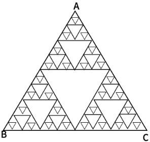
Since the triangle has a perfectly constant self-similarity and the number of triangles is constantly increasing based on the second largest triangle in the center, the center of gravity becomes the center of gravity of triangle ABC, and the center of gravity of this Sierpinski triangle Equal, that is, the center of gravity G is ((a+c+e)/3,(b+d+f)/3) when the corners are defined as A(a,b), B(c,d) and C(e,f), respectively.

2.1.2. Asymmetry

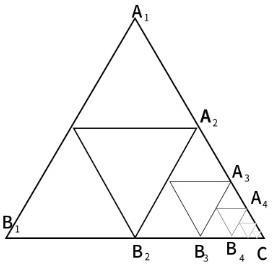
The center of gravity of the following triangle shown in fig.3 is the center of gravity G₁ of triangle A₁B₁C₁, the center of gravity G₂ of triangle A₂B₂C₂, the center of gravity G₃ of triangle A₃B₃C₃… The center of gravity of all the centers of gravity of each triangle up to the center of gravity G_∞ of triangle A_∞B_∞C_∞ will be the center of gravity of the entire triangle, and since all these centers of gravity are located in one straight line, the midpoint of the straight line that is the center of gravity of the straight line This will be the center of gravity.

2.2. Hexagon

2.2.1. Symmetry

Suppose each hexagon center of gravity (G) is treated as a point, and the center of gravity of all centers of gravity is obtained. In the case, the total center of gravity of the hexagonal model is obtained. That is, the center of gravity of the hexagonal tongue at the center becomes the center of gravity of the model.

2.2.2. Asymmetry

The center of gravity of this model can also be obtained using the same method as above. First, find the centers of gravity of each hexagon, then find the centers of gravity of the adjacent hexagons, and repeat this process to find the center of gravity of each point when it comes out, this is a model of the center of gravity.

2.3. Deformation process when force is applied to the research model

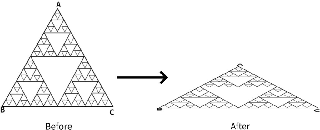
2.3.1. Triangle

Symmetry, force downward: This is the process of change when the triangle is pressed downward. To find the center of gravity like the previous front, you just need to set the coordinates of the vertices of each angle, but the center of gravity of the triangle before applying the force to the front is located above the center of gravity after pressing. In other words, whenever you press the button, the center of gravity moves downward like each point. Point A will gradually go downwards, and the two points B and C will spread apart due to the downward force. Therefore, to find the center of gravity, first set the midpoint of B C as the origin of the coordinate plane. Then point A will be on the y-axis and each B and C will be on the x-axis. If a downward force is applied, the x-coordinate of point A will be 0, the y-coordinate will gradually decrease from the starting point, and the absolute values of the coordinates of points B and C will increase, respectively. Using the formula to find the coordinates of the center of gravity, the x-coordinate is 0 because the sum of the x-coordinates of the point B and point C is 0, the point A is on the y-axis, so the y-coordinate is a point because the point B and C are on the x-axis We only need to care about the y-coordinate of A. The y-coordinate of point A gets smaller as the force is applied, so in conclusion, the center of gravity falls according to the amount of force applied.

Symmetry, compression by applying force from both sides: If the coordinate plane is set up the same way as before, point A is on the y-axis, and points B and C on the x-axis. This time, since it was compressed with the same force from both sides, the x-coordinate of point A remains 0.The y-coordinate increases, and since the points B and C have been pulled to the origin by the same distance, the y– coordinate remains 0, and the x-coordinate is their absolute value. This will decrease If you find the coordinates of the center of gravity with the formula for calculating the center of gravity. The x-coordinate increases due to the increase in the x-coordinate of point A, and the y-coordinate is 0. That is, the center of gravity moves upwards on the y-axis. the change in the center of gravity by finding the center of gravity of the asymmetric triangle No. 2. Let g be the center of gravity before applying the force, and let G be the center of gravity after applying the force. We will set the coordinate plane with b2 as the origin this time. When a downward force is applied and pressed, a1 descends downward along the y-axis, and each of the remaining b and c coordinates lengthens sideways. Now, we will explain the change in the center of gravity by finding the center of gravity. First, if the center of gravity of triangle A1 B1 C is G1, the coordinates of G1 will descend as force is applied, and the X coordinate of C will increase. This way, the center of gravity appears to be shifted diagonally in the lower right corner.

Asymmetric, press with force from both sides: If the center of gravity is changed using the method of finding the center of gravity of the asymmetric triangle No. 2, in this situation, the y coordinate of point A1 increases because force is applied and pressed from both sides The absolute value of each x coordinate of B1 and C is also gradually increased. Decreases A1 B1 C if the center of gravity of the triangle is G1, the coordinates of G1 rise upward as the force is applied, and point C moves to the left toward the origin. When looking at the movement of the two points, the center of gravity of the entire model shows a movement in the upper left direction.

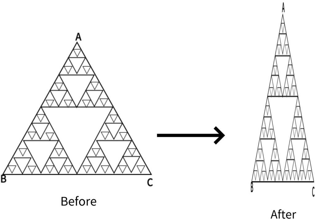
Asymmetric, press with downward force: We will show the change in the center of gravity by finding the center of gravity of the asymmetric triangle No. 2. Let g be the center of gravity before applying the force, and let G be the center of gravity after applying the force. We will set the coordinate plane with b2 as the origin this time. When a downward force is applied and pressed, a1 descends downward along the y-axis, and each of the remaining b and c coordinates lengthens sideways. Now, we will explain the change in the center of gravity by finding the center of gravity. First, if the center of gravity of triangle A1 B1 C is G1, the coordinates of G1 will descend as force is applied, and the X coordinate of C will increase. This way, the center of gravity appears to be shifted diagonally in the lower right corner.

Asymmetric, press with force from both sides: If the center of gravity is changed using the method of finding the center of gravity of the asymmetric triangle No. 2, in this situation, the y coordinate of point A1 increases because force is applied and pressed from both sides The absolute value of each x coordinate of B1 and C is also gradually increased. Decreases A1 B1 C if the center of gravity of the triangle is G1, the coordinates of G1 rise upward as the force is applied, and point C moves to the left toward the origin. When looking at the movement of the two points, the center of gravity of the entire model shows a movement in the upper left direction.

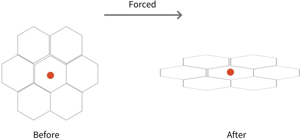
2.3.2. Hexagon

Symmetry, the downward force: Set the center of the two vertices of the following model as the origin, and set the coordinate plane so that the center of gravity (red dot) is on the y-axis. Because the model is pressed down, the overall height is lowered and spreads to the sides. Since the center of gravity of the following model coincides with the center of gravity of the regular hexagon in the center, only the change process of the center of gravity of the regular hexagon in the center needs to be examined. The center of gravity of a regular hexagon is the center of gravity of an equilateral triangle that connects the three adjacent vertices of the hexagon by one square. Therefore, to examine the change in the center of gravity of the angular shape in the center, only the change in the inner equilateral triangle is required. Therefore, it shows the same shape as the change in the center of gravity of 1-1-1. As the force is applied and pushed down, the center of gravity goes down on the y-axis. Symmetry, compression by applying force from both sides: Set the center of the two vertices of the following model as the origin and the coordinate plane so that the center of gravity (red point) is on the y-axis. Because it is compressed by applying force from both sides, the overall height increases and the sides are contracted. Since the center of gravity of the following model coincides with the center of gravity of the regular hexagon in the center, only the change process of the center of gravity of the regular hexagon in the center needs to be examined. The center of gravity of a regular hexagon is the center of gravity of an equilateral triangle that connects the three adjacent vertices of the hexagon by one square. Therefore, to examine the change in the center of gravity of the angular shape in the center, only the change in the inner equilateral triangle is required. This way, it shows the same shape as the 1-1-2 change in the center of gravity. As you apply force and compress it sideways, the center of gravity continues to rise upwards on the y-axis.

3. Method

The ceramic material is relatively light, hard, and has ex- cellent strength at a high temperature compared to other materials such as metal, and has excellent abrasion and corrosion resistance, so it is widely used as a core material for parts used at high temperatures, such as cutting tools, high-temperature parts, and gas turbine engine parts. Rep- resentative structural ceramic materials include oxide-based materials such as Al₂O₃ and ZrO₂ and non-oxide-based materials such as SiC, Si₃N₄, B₄C, AlN, and TiC. A ceramic component material used at a high temperature requires mechanical properties such as strength, elastic modulus, stress-deformation characteristics, etc., in a temperature environment used together with thermal properties such as thermal conductivity, specific heat, thermal expansion coefficient, etc. Generally, a method of measuring the modulus of elasticity of a material includes a direct method such as a tensile test and a 3-point or 4-point bending test [29, 30].

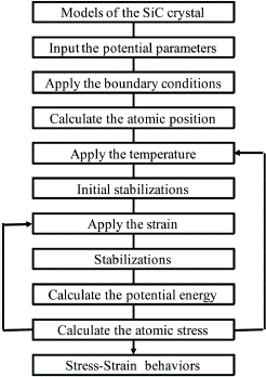
In addition, with the development of high-speed and large capacity of computers, computer simulation research has been actively conducted to analyze the microscopic behavior of atomic levels of materials using molecular dy- namics and first principles, and research is being conducted to analyze the properties of materials, such as modulus of elasticity.Suppose it is possible to predict the mechanical properties according to the temperature of the ceramic ma- terial using this. In that case, it will significantly help the design and the development of the ceramic part material for high temperatures [31].

Using molecular dynamics, this study analyzed the stress-displacement behavior and elastic modulus of SIC fractal crystals, which are high-temperature structural ma- terials at various temperatures.To this end, SiC crystals are modeled using Tersoff potential, and 1,2504oC from room

temperature using LAMMPS S/W, a high molecular dy- namics program [32]. We tried to analyze the change in elastic modulus according to temperature by analyzing the stress-displacement characteristics up to this point

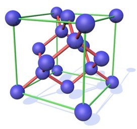
3.1. Interatomic bonding potential of SiC crystals

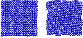
The unit cell structure of the SiC crystal is shown in Figure1. Here, the Si atom is located at each corner and face center in the lattice, and the C atom is located at the center of the tetrahedron based on the Si atom. In addition, atoms inside the SiC crystal may be arranged in the form of CC-C, C-C-Si, C-Si-Si, Si-Si-Si, C-Si-C, Si-C-Si, etc., and potential energy acting between adjacent atomic arrays is required.

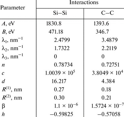
Tersoff developed potential energy that simulates the interatomic bonds of SiC crystals using classical interatomic potential. The Tersoff potential has been successfully used in the study of various related materials as a proposed po- tential to simulate bonds between elements with tetravalent covalent bonds of carbon, silicon, and germanium. Tersoff described the interaction of atoms as a potential energy function using the empirical bond-order concept. The ag- glomeration energy (E) of the object is described as follows in Equation (1) [33, 34].

$$E = \sum_i E_i + \frac{1}{2} \sum_{i \ne j} V_{ij} \tag{1}$$

4. Results and discussions

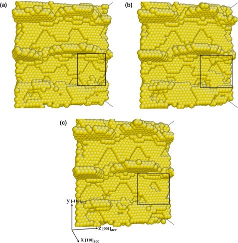
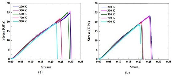
Before looking at the results and the contents of the discussion, I will briefly predict the results by looking at the experimental images from Figures 4 to 8. The difference between the strength of symmetry and the strength of asymmetry resulted in the symmetric model being more powerful than the asymmetric model. Figures 4 to 8 show the defor- mation process of a symmetrical triangle and a symmetrical hexagonal shape among the models that modeled the SiC crystal with a fractal model. First, Figure 4 shows the de- formation process at the beginning of applying force to a symmetrical triangle. When you look at the picture, you can find that the shape of the model breaking into a diagonal shape is relatively stable and regular. However, looking at the experimental image of the LAMMPS program in Figure 5, the changes to (a) (b) (c) are quite regular and stable, but since (c) most decisions have been broken in an instant, unlike the way they have been broken. On the other hand, looking at the experimental images of the symmetrical hexagonal LAMMPS program, all (a) to (h) show relatively regular changes that are destroyed after converging to stable constant values. Therefore, it showed a regular appearance to the end rather than a triangular model. This can be predicted as the first evidence that a symmetrical hexagon is more powerful in terms of stress/change and strength than a symmetrical triangle. When looking at the graph model in Figure 7, the same results as before are derived. However, the stress change graph of Young’s Modulus in Figure 8 yields slightly different results in the front tube. In(a) , the symmetrical triangle is examined in (b) for the changes in the symmetrical hexagon. However, when the temperature was raised to 900K in part (a), it could be seen that it was broken after holding it a little, but in part (b), it was bro- ken relatively faster than in (a) when it was raised to 900K. In addition, overall (a) showed superiority over (b) in all aspects.

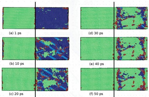
Stress-strain properties and modulus of elasticity were analyzed while changing the temperature of SiC crystals from room temperature to 1,500oC, and the results are shown in Figure. It is shown from 4 to Fig. 8. First, when the SiC crystal has triangular symmetry, the shape is deformed by the application of the compression displacement at 1,000oC.

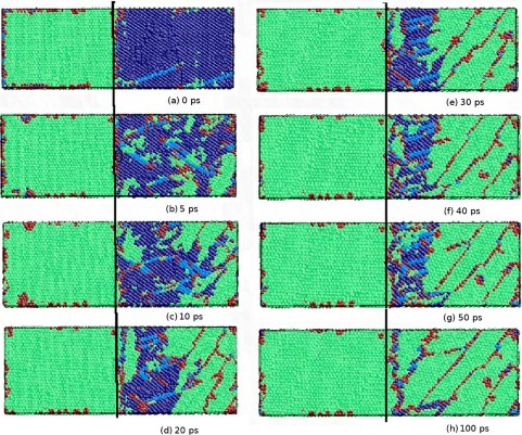
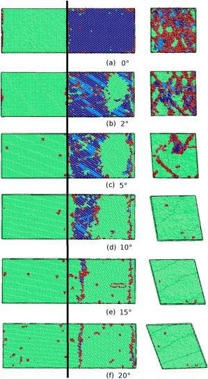
Fig. 4(a) shows the SiC crystal thermally stabilized at 1,000oC. Fig. 4(b) shows the deformed shape by applying the compression displacement of 0.15. In particular, when high compressive stress was applied at a temperature of 1,100oC or higher, it was confirmed that some outermost specific atoms of the SiC crystal significantly deviated from the unit lattice position. This is the thermal vibration of the active atoms at high temperatures. It is believed that some outermost atoms have deviated from the unit lattice position due to the combined high displacement energy applied. Therefore, the stress-displacement characteristics of SiC crystals are calculated by calculating the average stress of the internal unit lattice with only the members, except for atoms that deviate from the unit lattice position to improve the accuracy of the analysis. The modulus of elasticity was analyzed [35, 36].

The figure uses molecular dynamics to analyze the stress- displacement characteristics of SiC crystals with triangular symmetry at 1,000oC temperature. It is shown in 5. In this case of SiC crystals, the stress increases linearly as the total energy increases as the gap between atoms approaches due to the compression displacement. Furthermore, when a compression displacement of 0.2 or more was applied, the entire stress was destroyed after converging to a certain value. In addition, even if the crystal temperature increases to 500oC, SiC crystals exhibit stress-displacement characteristics similar to room temperature. However, if the temperature of the crystal increases by more than 1,000 oC, the SiC crystal will exhibit an inflection point similar to the elastic-plastic limit of yielding stress at a displacement of about 0.1. This result is entirely different from the result that ceramics such as SiC, which are known so far, are destroyed after elastic deformation. However, it is judged that additional analysis is needed to suggest that SiC crystals may also undergo plastic deformation at high temperatures.

Changes in the modulus of elasticity of crystals with broken symmetry were also investigated using molecular dynamics from the stress-displacement characteristics of SiC with triangular symmetry. The modulus of elasticity of SiC crystals with broken symmetry is shown. It was found that it was about 475 GPa at room temperature and decreased to about 425 GPa as the temperature increased to 1,250oC.

5. Conclusion

SiC ceramics are excellent materials applied at high temperatures because of their light- weight, excellent high- temperature strength, and high thermal shock resistance. Data on stress-strain characteristics and modulus of elasticity depending on temperature are required to design a ceramic for a high temperature structure, but it is challenging to measure them. This study analyzed the elastic modulus characteristics of SiC crystals at various temperatures using molecular dynamics. To this end, SiC crystals were modeled to apply Tersoff potential between constituent atoms, and stress-strain behavior and modulus changes from room temperature to 1,250oC were analyzed using LAMMPS S/W, a molecular dynamics program. As a result of this study, it was confirmed that the modulus of elasticity of SiC crystals changed in the range of about 475 GPa to 425 GPa as it increased from room temperature to 1,250 oC. The stress- displacement characteristics of SiC crystals, which could not be measured at a high temperature of 1,000 oC or higher, could be ensured.

1. B. B. Mandelbrot, B. B. Mandelbrot, The fractal geometry of nature, https://doi.org/10.1002/bbpc.19850890223, vol. 1, WH freeman New York, 1982.
2. B. B. Mandelbrot, D. Passoja, A. J. Paullay, et al., “Fractal character of fracture surfaces of metals, https://doi.org/10.1038/308721a0”, Nature, vol. 308, no. 5961, pp. 721–722, 1984.
3. M. F. Barnsley, R. L. Devaney, B. B. Mandelbrot, H.-O. Peitgen, D. Saupe, R. F. Voss, Y. Fisher, M. McGuire, The science of fractal images, https://doi.org/10.1007/978-1-4612-3784-6, vol. 1, Springer, 1988.
4. B. B. Mandelbrot, “Fractal geometry: what is it, and what does it do?, https://doi.org/10.1098/rspa.1989.0038”, Proceedings of the Royal Society of London. A. Mathematical and Physical Sciences, vol. 423, no. 1864, pp. 3–16, 1989.
5. B. B. Mandelbrot, C. J. Evertsz, M. C. Gutzwiller, Fractals and chaos: the Mandelbrot set and beyond, https://doi.org/10.1007/978-1-4757-4017-2, vol. 3, Springer, 2004.
6. P. H. Coleman, L. Pietronero, “The fractal structure of the universe, https://doi.org/10.1016/0370-1573(92)90112-d”, Physics Reports, vol. 213, no. 6, pp. 311–389, 1992.
7. T. Hirata, “Fractal dimension of fault systems in japan: fractal struc- ture in rock fracture geometry at various scales, doi: 10.1007/978- 3-0348-6389-6_9”, “Fractals in geophysics”, pp. 157–170, Springer, 1989.
8. H. V. Meyer, T. J. Dawes, M. Serrani, W. Bai, P. Tokarczuk, J. Cai, A. de Marvao, A. Henry, R. T. Lumbers, J. Gierten, et al., “Genetic and functional insights into the fractal structure of the heart, https://doi.org/10.1038/s41586-020-2635-8”, Nature, vol. 584, no. 7822, pp. 589–594, 2020.
9. T. Higuchi, “Approach to an irregular time series on the basis of the fractal theory, https://doi.org/10.1016/0167-2789(88)90081-4”, Physica D: Nonlinear Phenomena, vol. 31, no. 2, pp. 277–283, 1988.
10. S. Frontier, “Applications of fractal theory to ecology doi: 10.1007/978- 3-642-70880-0_9”, “Develoments in numerical ecology”, pp. 335–378, Springer, 1987.
11. A. Le Méhauté, Fractal Geometries Theory and Applications, https://dl.acm.org/doi/abs/10.5555/153370, CRC Press, 1991.
12. E. Fernández, H. F. Jelinek, “Use of fractal theory in neu- roscience: methods, advantages, and potential problems, https://doi.org/10.1006/meth.2001.1201”, Methods, vol. 24, no. 4, pp. 309–321, 2001.
13. K. Falconer, Fractal geometry: mathematical foundations and applications, DOI:10.1002/0470013850, John Wiley & Sons, 2004.
14. G. Captur, A. L. Karperien, A. D. Hughes, D. P. Francis, J. C. Moon, “The fractal heart—embracing mathematics in the cardiology clinic, https://doi.org/10.1038/nrcardio.2016.161”, Nature Reviews Cardiology, vol. 14, no. 1, pp. 56–64, 2017.
15. M.-L. De Keersmaecker, P. Frankhauser, I. Thomas, “Using fractal dimensions for characterizing intra-urban diversity: The example of brussels, https://doi.org/10.1111/j.1538-4632.2003.tb01117.x”, Geographical analysis, vol. 35, no. 4, pp. 310–328, 2003.
16. J. Fleckinger-Pellé, D. G. Vassiliev, “An example of a two- term asymptotics for the “counting function” of a fractal drum, https://doi.org/10.1090/s0002-9947-1993-1176086-7”, Transactions of the American Mathematical Society, vol. 337, no. 1, pp. 99–116, 1993.
17. S. Bleher, C. Grebogi, E. Ott, R. Brown, “Fractal boundaries for exit in, https://doi.org/10.1103/physreva.38.930”,
    al Review A, vol. 38, no. 2, p. 930, 1988.
18. J. A. Riousset, V. P. Pasko, P. R. Krehbiel, R. J. Thomas, W. Rison, “Three-dimensional fractal modeling of intracloud lightning discharge in a new mexico thunderstorm and comparison with lightning map- ping observations, https://doi.org/10.1029/2006jd007621”, Journal of Geophysical Research: Atmospheres, vol. 112, no. D15, 2007.
19. J. Valdivia, G. Milikh, K. Papadopoulos, “Red sprites: Lightning as a fractal antenna, https://doi.org/10.1029/97gl03188”, Geophysical Research Letters, vol. 24, no. 24, pp. 3169–3172, 1997.
20. R. S. Snow, “Fractal sinuosity of stream channels, https://doi.org/10.1007/bf00874482”, Pure and applied geophysics, vol. 131, no. 1, pp. 99–109, 1989.
21. P. La Barbera, R. Rosso, “On the fractal dimension of stream networks, https://doi.org/10.1029/wr025i004p00735”, Water Resources Research, vol. 25, no. 4, pp. 735–741, 1989.
22. C. Puente, J. Claret, F. Sagues, J. Romeu, M. Lopez-Salvans, R. Pous, “Multiband properties of a fractal tree antenna generated by electro-chemical deposition, 10.1049/el:19961579”, Electronics Letters, vol. 32, no. 25, pp. 2298–2299, 1996.
23. P. Perdikaris, L. Grinberg, G. E. Karniadakis, “An effective fractal-tree closure model for simulating blood flow in large arterial networks, https://doi.org/10.1007/s10439-014-1221-3”, Annals of biomedical engineering, vol. 43, no. 6, pp. 1432–1442, 2015.
24. R. R. Bradbury, R. R. Reichelt, et al., “Fractal dimension of a coral reef at ecological scales, doi:10.3354/meps010169”, Marine Ecology Progress Series-pages: 10: 169-171, 1983.
25. D. M. Mark, “Fractal dimension of a coral reef at ecological scales: a discussion, https://doi.org/10.3354/meps014293”, Marine ecology Progress series, vol. 14, pp. 293–294, 1984.
26. B. Martin-Garin, B. Lathuilière, E. P. Verrecchia, J. Geis- ter, “Use of fractal dimensions to quantify coral shape, https://doi.org/10.1007/s00338-007-0256-4”, Coral Reefs, vol. 26, no. 3, pp. 541–550, 2007.
27. R. F. Cahalan, J. H. Joseph, “Fractal statistics of cloud fields, https://doi.org/10.1175/1520-0493(1989)117<0261:fsocf>2.0.co;2”, Monthly weather review, vol. 117, no. 2, pp. 261–272, 1989.
28. N. Sánchez, E. J. Alfaro, E. Pérez, “On the properties of fractal cloud complexes, 10.1086/500351”, The Astrophysical Journal, vol. 641, no. 1, p. 347, 2006.
29. S.-H. Kim, “Fractal dimensions of a green broccoli and a white cauliflower, doi: 10.1093/cercor/6.6.830”, arXiv preprint cond- mat/0411597, 2004.
30. M. Peleg, G. V. Barbosa, “Fractals and foods, https://doi.org/10.1080/10408399309527617”, Critical Reviews in Food Science & Nutrition, vol. 33, no. 2, pp. 149–165, 1993.
31. J. González, A. Gamundi, R. Rial, M. C. Nicolau, L. de Vera, E. Pereda, “Nonlinear, fractal, and spectral analysis of the eeg of lizard, gallo- tia galloti, doi: 10.1152/ajpregu.1999.277.1.r86”, American Journal of Physiology-Regulatory, Integrative and Comparative Physiology, vol. 277, no. 1, pp. R86–R93, 1999.
32. F. Chen, K. Wang, B. Shi, H. Hu, “Dendrite and fractal patterns formed on the surface of bismuth-ion-implanted linbo3, doi:10.1088/0953- 26/304”, Journal of Physics: Condensed Matter, vol. 13, no. 26,
    3, 2001.
33. A. S. Priya, D. Geetha, Ş. Ţălu, “Advanced micromor- phology study of the mn-doped bismuth ferrite thin films, https://doi.org/10.1016/j.matlet.2020.128615”, Materials Letters, vol. 281, p. 128615, 2020.
34. F. E. Lennon, G. C. Cianci, N. A. Cipriani, T. A. Hensing, H. J. Zhang, C.-T. Chen, S. D. Murgu, E. E. Vokes, M. W. Vannier, R. Salgia, “Lung cancer—a fractal viewpoint, doi: 10.1038/nrclinonc.2015.108”, Nature reviews Clinical oncology, vol. 12, no. 11, pp. 664–675, 2015.
35. T. Nelson, B. West, A. Goldberger, “The fractal lung: universal and species-related scaling patterns, doi: 10.1007/bf01951755”, Experien- tia, vol. 46, no. 3, pp. 251–254, 1990.
36. Y.-T. Zuo, H.-J. Liu, “Fractal approach to mechanical and electrical properties of graphene/sic composites, 10.22190/fume201212003z”, Facta Universitatis. Series: Mechanical Engineering, vol. 19, no. 2, pp. 271–284, 2021.
37. C. Atzeni, G. Pia, U. Sanna, “Fractal modelling of medium–high poros- ity sic ceramics, https://doi.org/10.1016/j.jeurceramsoc.2008.03.039”, Journal of the European Ceramic Society, vol. 28, no. 14, pp. 2809–2814, 2008.
38. B. Li, Z. Chen, E. Ren, “A fractal analysis for the microstructures of β-sic films, https://doi.org/10.3139/146.111802”, International Journal of Materials Research, vol. 110, no. 8, pp. 746–756, 2019.
39. M. T. Humbert, Y. Zhang, E. J. Maginn, “Pylat: Python lammps analysis tools, doi:10.1021/acs.jcim.9b00066”, Journal of chemical information and modeling, vol. 59, no. 4, pp. 1301–1305, 2019.
40. P. G. Mezey, “Potential energy hypersurfaces, https://doi.org/10.1016/b978-044452227-6/50015-6”, 1987.
41. E. N. Lorenz, “Available potential energy and the maintenance of the general circulation, https://doi.org/10.1111/j.2153- 3490.1955.tb01148.x”, Tellus, vol. 7, no. 2, pp. 157–167, 1955.
42. S. Ito, M. Hashimoto, B. Wadgaonkar, N. Svizero, R. M. Carvalho,C. Yiu, F. A. Rueggeberg, S. Foulger, T. Saito, Y. Nishitani, et al., “Effects of resin hydrophilicity on water sorption and changes in modulus of elasticity, doi: 10.1016/j.biomaterials.2005.04.052”, Biomaterials, vol. 26, no. 33, pp. 6449–6459, 2005.
43. A. Pauw, Static modulus of elasticity of concrete as affected by density, University of Missouri, 1960. https://doi.org/10.3390/ma14247578,

Citations by Dimensions

Citations by PlumX

Crossref Citations

This paper is currently not cited.

No. of Downloads per Month

No. of Downloads per Country