This research is about tuning the automatic generator control (AGC) unit within the National Transmission System (NTG) and is intended to provide a set of key insights into problems related to generator control systems oscillations and the possible available solutions. The case study is the Baba Hydroelectric Power Plant in Ecuador. The aim is to model, simulate and validate the controls of the Baba generating units for an optimal and stable response. Both controllers, the Automatic Voltage Regulator (AVR) and Power System Stabilizer (PSS) were tuned using both a component-based approach using an object-orientated tool where the model structure resembles the original system, and a coexisting power flow tool in a signal orientated environment. A key part of this tuning is the adaptation of the model to different operating conditions by testing scenarios where signals ought to be defined before the start of the simulation and others be chosen for visualisation without any limitation, therefore, this paper is about finding a multi-framework environment. Also, the model was disturbed so to observe the field Voltage and terminal voltage values using a simplified and reduced part of the NTG. Results show that a high gain AVR helps the steady state and transient stabilities but may reduce the oscillatory stability and the PSS can provide significant stabilization of such oscillations. The validation strategy uses the average quadratic mean square error statistical method.

1. Introduction

Hydroelectric power plants are the foundation of Ecuador’s power generation capacity. Hydropower plants account for 57.67% [1] of the country’s installed capacity by 2017. Our case study is the Baba Multi-Purpose Project (BMP), consisting of four dikes and three channels in Los Ríos province, used for irrigation, flood control, water supply and hydroelectric power generation. The BMP includes water supply to the reservoir and the Daule-Peripa reservoir, construction of the hydroelectric power plant and associated transmission lines. Therefore, the main purpose of the BMPs is water storage and transmission, not hydropower. Upland rice is dominant in Los Rios and no-tillage is the dominant crop cultivation method. About 60 percent of the farmers farm less than five hectares per person and three percent are large farmers cultivating 100 hectares per person [2]. With 3,000 hectares of land at risk of flooding, protesters against the Baba dam had a major impact on the construction of the dam and saved the community from flooding [3]. Capable of generating 42 MW, covering 40-50% of the demand in Los Ríos. The Baba hydropower station has two of his Kaplan direct shaft turbines submerged by a spiral cover or scroll area.

This paper concerns the feasible enhancement controls which may allow the countrywide electricity grid to perform reliably over broader tiers of loading and system operational point. Hydro-turbines controllers are tuned for assumed situations withinside the relaxation of the electricity grid; however, as grid situations vary, the controllers eventually ‘malfunction’ in one-of-a-kind ways (ranging being too sluggish and/or of inadequate ability or loss of coordination) [4]; consequently, it is hard to ensure system-wide performance; therefore, the general tendency is not to rely on control outside normal regions and find out where are the opportunities to operate efficiently. A method is wanted for dealing with the machine throughout a huge variety of running condition, for this is important to display electricity-flows and adjust those consistent with the higher described generator interconnection standards making sure viable electricity exchanges without compromising machine reliability; however, at the same time, the design has to be completed in order that every generator maintains its decentralized, self-sufficient operation, whilst coordinating with turbines of the nearby electricity grid.

Literature review shows different ways authors can implement controls. For example, Std 421.5™-2005 [5] describes a model structure intended to facilitate the use of field test data as a means of obtaining model parameters. In North America model validation is mandated according to the Reliability Council (NERC) Modelling, Data, and Analysis (MOD) series of standards. NERC MOD-033-1 [6] specifies consistent validation requirements to facilitate the collection of accurate data and the development of planning models for reliability analysis of interconnected transmission systems. In Europe, [7] designed a robust controller to address both local area and inter-area oscillations. The controller is a second-order state-space regulator. In Ecuador, [8] is developing tools for displaying oscillation modes and their damping, and for provisional localization of a PSS in the Ecuadorian NTG. An online model estimation scheme was also used to validate and/or tune a small-signal model of the power system using synchro phasor data [9] at the Paute-Molino power plant in Ecuador [10]. In Modelica [11] there was an effort on design principles and a prototype for modelling the pan-European electricity grid to be used by European transmission system operators.

The controls are an Automatic Voltage Regulator (AVR) and a Power System Stabilizer (PSS). The AVR regulates the terminal voltage of the generator. A fast-response high-gain AVR improves large-signal transient stability in the sense that it improves the network’s ability to maintain synchronism when subjected to severe transient disturbances. There is a trade-off between synchronous torque provided by the AVR and the damping torque provided by the PSS [12,13]. PSS tuning is for a wide oscillation damping applications. PSS requires a reliable model of the system in a software package such as DigSILENT PowerFactory (PF). The early stages of this research involved extensive data management, cleansing, and restructuring to the NTG initial dataset in the PF package. The development of these controllers uses an object-oriented and non-causal modelling approach in which individual parts of the model are directly described as equations using a declarative approach [14] but also coexisting in good cooperation with signal-orientated tools.

2. Methodology

2.1. Generation unit modelling

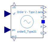
The Baba power generation unit will generate 161 GWh/year by pumping water to the Santa Elena Peninsula at up to 234 m³/sec. During the rainy season (January to October), the reservoir only provides a downstream flow of 10 – 15 m³/sec. The generating units are two horizontal axis Kaplan turbines, each of 21 MW, with a maximum operating flow of 86 m³/ sec. The difference from the maximum flow rate, approximate 62 m³/sec, is discharged via a by-pass installed next to the pressure line [15]. Clarke and Park transforms are commonly used in field-oriented control of three-phase AC machines. The Clarke transform converts the time domain components of a three-phase system (in abc frame) to two components in an orthogonal stationary frame (ab). The Power System Analysis Toolbox (PSAT) hydroelectric salient pole machine is modelled as Order V Type 2 model [16], which more closely resembles the Baba generator characteristics. Both follows Van-Cutsem and Papangelis [17] proposed data (see Figure 1). Baba generator parameters and initial NTG values are shown in Table 1. The internal parameters of the generator are the same for Isolated and in NTG operation modes, but their initialization values differ depending on the controller’s mode of operation. Table 1 also shows the initial values for the Isolated – NTG generator. To view the controller’s response, a voltage disturbance in the form of a pulse generator was applied to the V_ref input. The ‘Pulse Generator’ parameters are shown in Table 2.

The generation model corresponds to a three-phase synchronous generator and a classic electromechanical model with transfer functions to model the direct and quadrature inductances. Assuming an additional circuit for the direct axis, the state variables can be described as in the following equations [18]. A curious reader would have to read the GitHub repository for all the models and parameters used from the OpenIPSL library.

The Model Parameters are Synchronous reactance – d axis (pu) Xd, Synchronous reactance – q axis (pu) X_q, Sub-transient reactance – d axis (pu) X_2d, Open circuit transient time constant – d axis (pu) T_1d0, Open circuit sub-transient time constant – d axis (pu) T_2d0, Open circuit sub-transient time constant – q axis (pu) T_2q0, Nominal Power (MVA) S_n, Nominal Voltage (kV) V_n, Armature Resistance (pu) R_a, Transient Reactance – d axis (pu) X_1d, Mechanical inertia coefficient M and Damping D.

Table 1: Parameters of the Baba Generator

Table 2: Parameters of the pulse generator

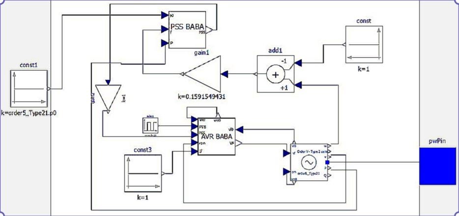
AVR modelling is in Section 2-2 and PSS is in Section 2-3. The closed-loop response has two outputs, P (power) and w (velocity), which are connected to the corresponding inputs of the PSS. A frequency f block was added that allows to change the speed to frequency and therefore being able to meet the number of equations and unknowns for the Generator validation. Enhancements have also been made to the PSS output to address what-if scenarios. The internal block diagram is shown in Figure 2 and the external block diagram is shown in Figure 3.

2.2. AVR Modelling

The IEEE 421.5 standard [5] is the IEEE recommended practice for excitation system models for power system stability studies. The models apply for frequency deviations of ±5\% from nominal frequency and oscillation frequencies up to 3 Hz. The Baba excitation system follows the IEEE 421.5 ST6B model. The AVR is shown in Figure 4 and consists of a field voltage regulator and a PI voltage regulator with a feedforward control in the inner loop. The field voltage controller implements proportional control.

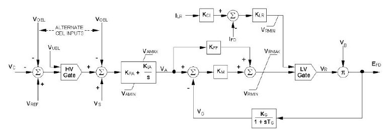
The AVR appeared in Figure 4 comprises of a PI voltage regulator with an internal loop field voltage regulator and pre-control. The field voltage regulator executes a proportional control. The pre-control and the delay in the feedback circuit increase the dynamic response. VR represents the limits of the power rectifier. The ceiling current IFD limitation is included in this model. The power for the rectifier, VB, may be supplied from the generator terminals or from an independent source. Inputs are provided for external models of the over-excitation limiter (VOEL), under-excitation limiter (VUEL), and PSS (VS).

Baba has a static excitation system in which the generator stator voltage is rectified by a thyristor bridge. This DC excitation voltage is fed through the slip ring to the rotor windings to excite the rotor. As the energized rotor rotates within the stator, an AC voltage is generated at the stator terminals, i.e., stator voltage variations directly affect the excitation voltage. Figure 5 shows the main exciter structure underlying the exciter modelled in the simulation tool.

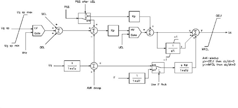
The variables and parameters in Figure 5 are the maximum allowed AVR reference U_{g sp max} (VHZ), the minimum allowed AVR reference U_{g sp min}, the transducer time constant T_u, field current time constant T_f, proportional gain K_p, integral time T_i, derivative gain K_d, derivative time constant T_d, Field current I_f, Use If the feedback in the loop control Use I_{f fdbck}, PSS after UEL, Field undercurrent limiter output MCLF, overdrive limiter output OEL, overdrive fast limiter output OEL_f, AVR compensation loop output AVR droop, Stator current limiter output SCL, Under-drive Limiter Output UEL, PSS output signal PSS, Volts hertz limiter output VHz. Typical parameter values are U_{g sp max} 1.1, U_{g sp min} 0.9, T_u 20 ms, T_f 20 ms, K_p 10, T_i 2 s, K_d 0, T_d 5 s, Use I_{f fdbck} 0 (Only for brushless excitation systems), PSS after UEL 1.

Our research focuses on damping of small signal swings, so we have simplified Figure 5. It is important to model the limiter in conjunction with the voltage regulator. Under excitation limiting is especially used in turbo generators. This is because without a limiter the reactive power output from the generator could be too high, leading to erroneous simulation results. Small turbo generators connected to powerful networks are sensitive to this kind of phenomenon [20]. The purpose of the over-excited limit is to protect the generator from overheating due to prolonged field over-current.

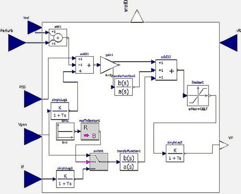
Figure 6 is a simplified non-causal AVR approach to modelling the Baba excitation system. Traditional approaches are based on block-oriented schemes in which causality plays a key role. However, new concepts based on object-oriented approaches, physics-oriented connections, and algebraic manipulation enable non-causal modelling, where blocks represent the interactions of equations.

Each of the transfer functions (TF) in Figure 6 has initialization parameter calibrated to stable values according to its response, either isolated or NTG modes. See Table 3.

Table 3: TF Initialization Isolated – NTG modes

The AVR’s operating parameters are adjusted according to a manufacturer’s specified ranges and are shown in Table 4.

Table 4: Isolated and NTG AVR Parameters

2.3. PSS Modelling

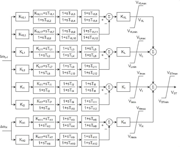
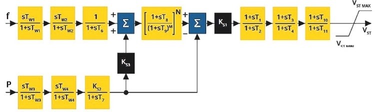
The IEEE 2005 421.5 standard [5] introduced a PSS structure called IEEE PSS4B. The PSS4B model represents a structure based on multiple operating frequency bands, as shown in Figure 7. Three separate bands, each dedicated to the low-, medium- and high-frequency oscillations modes, are used in the delta-omega (velocity input). Baba uses the IEEE Std 421.5^TM-2016 Dual-Input Power System Stabilizer (PSS₂C) [21] to improve electrical system stability, as shown in Figure 8. A key element is the Limiter. The Limiter is used to keep the PSS output voltage within a range of values and the PSS output protection should also match the output limiter. Additional damping can be achieved to improve transient stability by setting the PSS output limit. As a result, the PSS performance improves under larger system disturbances [22].

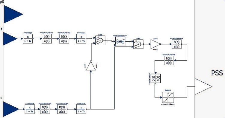
The PSS controller has a large number of ‘simple lag’ and ‘TransferFunction’, constants, limiters, input and output signals. It also has a ‘RampTrackingFilter’ for attenuating the signal. Non-casual modelling is shown in Figure 9.

Each of the transfer functions (TF) of Figure 9 have initialization parameters calibrated to stable values according to their response either isolated or NTG modes. See Table 5.

Table 5: TF Initialization Isolated — NTG modes

The operating parameters of the PSS were adjusted according to the ranges specified by the manufacturer. Parameters are shown in Table 6. PSS_min is equal to zero.

Table 6: Isolated and NTG PSS Parameters

In addition, the PSS controller is not a separate controller that is used with the generator, but it is a controller that input signals to the AVR by entering a signal into the AVR to improve the response after a failure.

2.4 National Transmission Grid

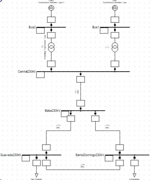
The early stages of this research involved extensive data management, cleansing, restructuring and additions to this initial dataset. In addition, real time test values of power flows were available via a robust PF power system tool. Figure 10 shows a reduced portion of the NTG with synchronous machines, transformers, transmission lines and system buses.

2.5 Transformers

Two elevating transformers (13.8:230 kV) were used for the implementation of the reduced grid. The transformer is connected to the synchronous generator. The primary winding of each transformer is connected to the generator’s armature winding at 13.8 kV. A circuit breaker is installed close to transformer on the upper (230 kV) voltage side. In this arrangement any generator perturbations and grid disturbances have an effect on the transformers. Transformers implemented in our system does have serial reactance and do not have iron losses. The transformer connection is grounded wye – delta. The grounded connection will provide a path for a line-to-ground fault current (back feed current) for a fault upstream from the transformer. The parameters are shown in Table 7.

Table 7: Transformers parameters

Simulation tools like PF facilitates the user with varied types of power system studies. It also obtains more detailed and accurate power-flow simulation solutions. However, the libraries integrated in the tools are normally closed for modifications. The values of power-flow that are entered in the non-causal model of transformers, generator, transmission lines and buses are acquired from PF.

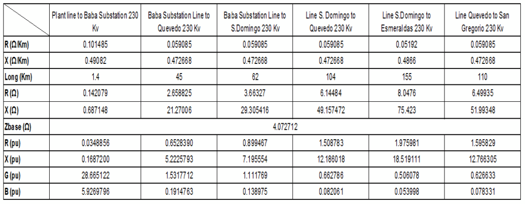
2.6 Transmission Lines

A NTG transmission line is modelled with an equivalent Õ circuit in the non-casual tool. The resistance (R) data is entered, whereas reactance (X), conductance (G) and susceptance (B) are obtained from DIgSILENT’s NTG block. All values are in p.u, but the units in PF are W/km and need to be converted using the Zbase into per unit. Zbase is calculated from Equation 1.

 $$Z_{base} = \frac{V^2}{P} = \frac{13{,}800^2}{46{,}760{,}000} = 4.072712\ [\Omega]\tag{1}$$

Zbase allows to compute all the lines from a reduced Baba grid. The line parameters are shown in Figure 11.

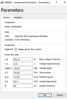
2.7 Infinite Buses

An infinite bus is the main bus of a power system with constant frequency and voltage (both in magnitude and angle). This research analyses the problem of a machine connected to an infinite bus via a transmission line. In general, fast excitation systems are usually beneficial to transient stability following large impacts by driving the field to fast response without delay. However, these abrupt changes in excitation are not necessarily beneficial in damping the oscillations that follow the first swing, and they sometimes contribute growing oscillations several seconds after the occurrence of a large disturbance [23]. We properly design the exciter as a mean of enhancing stability in the dynamic range as well as in the first few cycles after a disturbance. We consider two infinite bus implementations: the Esmeraldas and San Gregorio 230 kV buses. Input power-flow data for the non-casual system in those buses were from PF and is shown in Figure 12 for Esmeraldas as an example.

2.8 Equivalent system in OpenModelica

To illustrate the effect of the excitation system on transient stability, we perform transient stability study on the equivalent system shown in Figure 13.

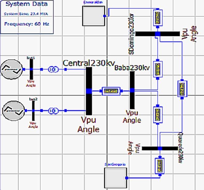
Figure 13 is the result after adding all the elements described in Sections 2.1 to 2.6. The generation parameters have been checked and AVR and PSS controller initialization values have also been adjusted as they are different from those in isolate mode.

Section 3-1 and Section 3-2 present the results and validation respectively of the system response. Validation tests are intended to later test the sensitivity estimates (see Section 3-4) derived from non-causal and causal approaches. This particular type of sensitivity analysis is being used in medicine [24]. Sensitivity helps identify potential risks in the power system.

3. Results

Related tests were performed on the Baba generation, including the AVR and PSS schemes shown in Figure 14. A gain follows the PSS output (‘gain2’ block in Figure 14) and also tracks frequency changes at the PSS input (‘add1’ block in Figure 14), both to understand the effect on the system response.

3.1 Isolated test results

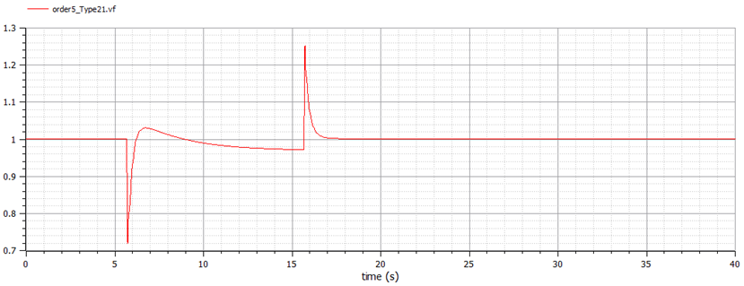
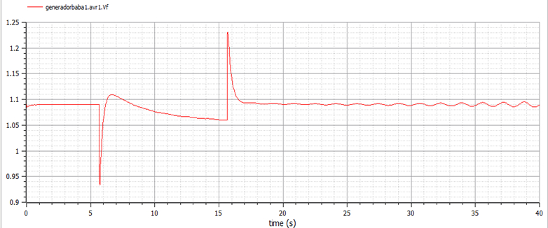
An isolated test of the controller was performed using a 10 second pulse train with amplitude -0.03 starting at 5.65 seconds, so the system returns to normal in 15.65 seconds. The field voltage response under these conditions is shown in Figure 15. In this figure, ‘gain2’ is set to zero to show only-AVR isolated field and terminal voltages responses.

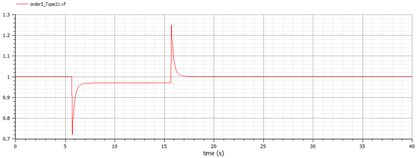
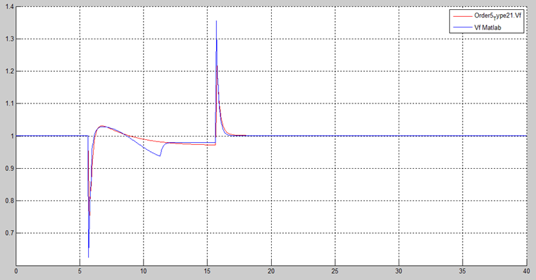
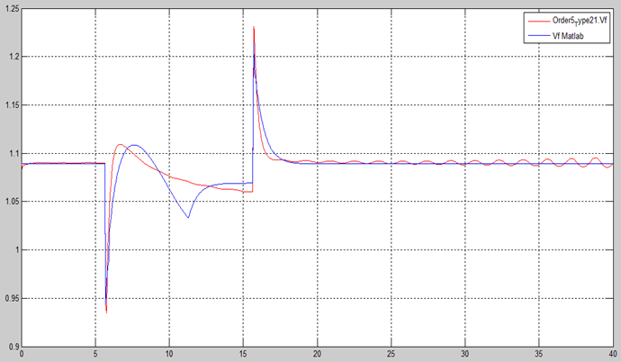
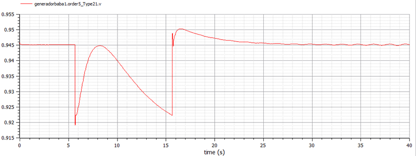
Figure 15 shows a stable response with a final value of 0.97 pu. Figure 16 shows the non-causal (red curve) and causal (blue curve) electric field voltage responses. Figure 16 shows that both curves are similar. A more detailed analysis of the differences using the mean squared error method follows in Section 3.4.

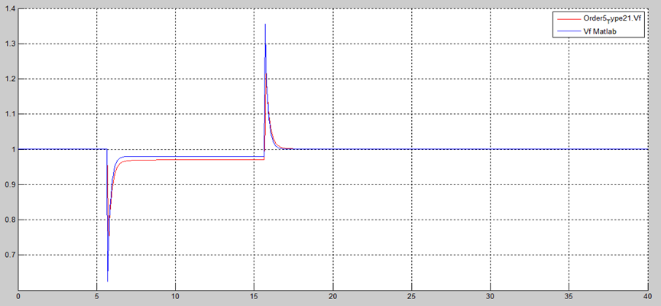
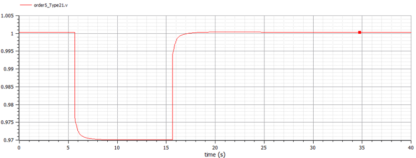
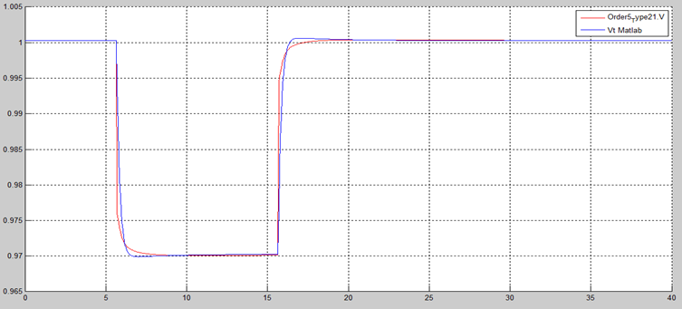
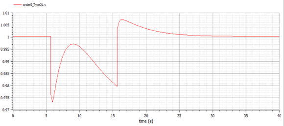
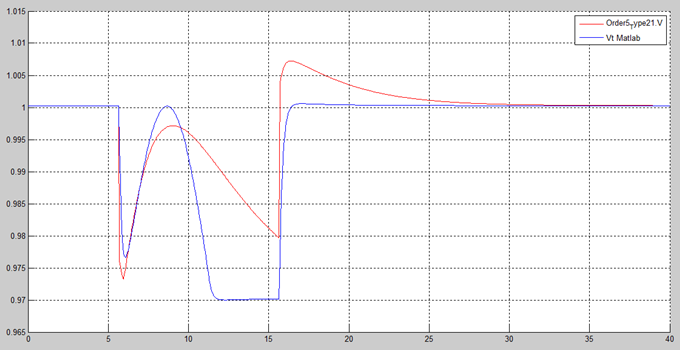
Figure 17 shows the terminal voltage (non-causal mode) with the same disturbance as it has a stable response with the electric field voltage. Figure 18 shows a comparison of the terminal voltage responses in the non-causal mode (red curve) and the causal model (blue curve).

By changing ‘gain2’ from zero to one, Figure 19 shows the isolated AVR + PSS field voltage response. Figure 19 shows stable response. Figure 20 shows a comparison of the electric field voltage responses of the non-causal (red curve) and causal models (blue curve) of AVR + PSS. These differences are not relevant.

The AVR + PSS voltage response is shown in Figure 21 and the comparison is shown in Figure 22. Similar to the field voltage response, there is a stable response and small voltage difference between non-causal and causal modes.

In summary, this Section demonstrates the effectiveness of AVR-only and AVR + PSS controllers. This result demonstrates the effectiveness of a fast-response, high gain AVR controller in reducing the power system oscillation stability, thereby improving its transient stability. On the other hand, the AVR + PSS controller reduces transient stability by overriding the voltage signal to the exciter to improve oscillation stability. Basically, the AVR and PSS controller actions are dynamically linked as expected.

In conclusion, both non-causal and causal modes are equally suitable. This reflects the fact that either approach can be used to create schematics of large power grids, once the hard work of creating a model suitable for simulation is completed. Random changes in model parameters are straightforward in the physical (non-causal) declarative equation-based mode.

3.2 NTG results

This Section shows the NTG field voltages and terminal voltages using the infinitive bus described in Section 2.7. An equivalent schema is shown in Figure 13. The same disturbances are used as for the isolated test, i.e., start at 5.65 seconds with and amplitude equal to -0.03 using a pulse train of one period. Figure 23 shows the NTG field voltage in the non-causal model using the AVR controller and Figure 24 shows the AVR field voltage comparing the non-causal and causal responses. Figures 23 and 24 show a stable response.

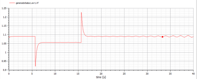
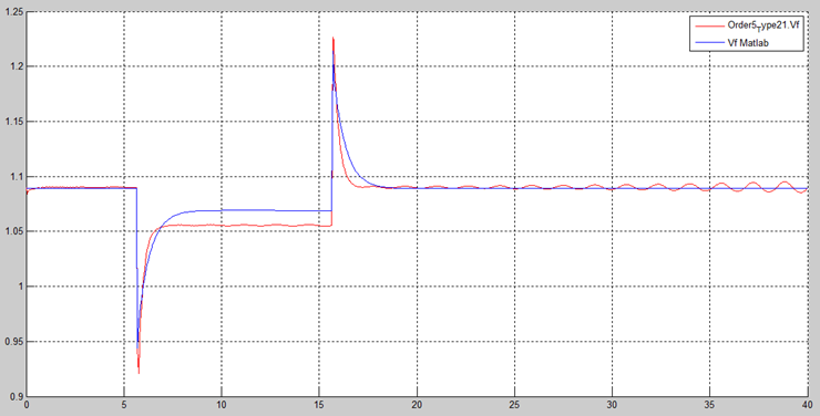
Figure 25 shows the terminal voltage response of the NTG AVR in non-causal mode and Figure 26 shows the NTG AVR response comparing non-causal and causal modes. Figures 25 and 26 show a stable response.

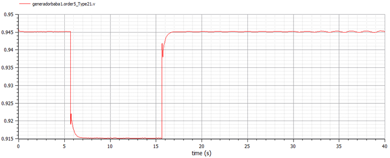
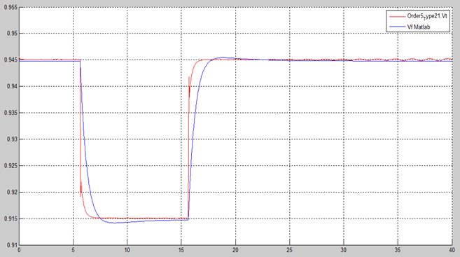
Figure 27 shows the NTG AVR + PSS field voltage response. Figure 28 shows the comparative non-causal – causal of the NTG field voltage. Figures 27 and 28 show a stable response.

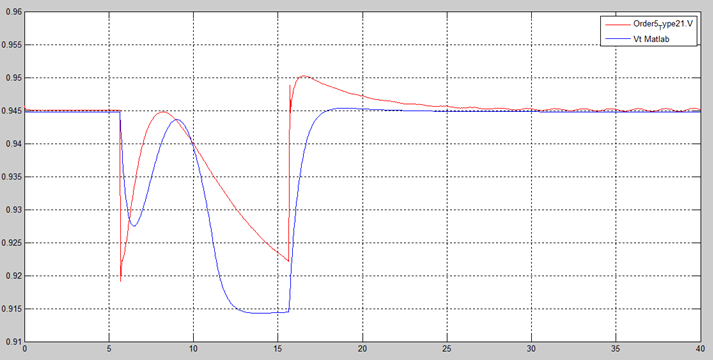
Finally, Figure 29 shows the terminal voltages of NTG AVR + PSS in a non-causal mode, and Figure 30 shows a comparison of terminal voltages in non-causal and causal modes. From Figures 29 and Figure 30 show a stable response.

The execution time is proportional to its complexity i.e., NTS case study simulation time is longer as expected for the same computer power (see Table 8).

Table 8: Simulation time

In summary, in the Ecuadorian NTG has many disturbances that affect the power grid and can affect the generator reliability. Some disturbances are from large loads. When a large load is suddenly connected to the power grid, the power demand increases as shown in the diagrams of this Section. When a load is suddenly added, the Baba generator frequency begins to oscillate. In the case of small load, oscillation can be damped quickly. Figures of this Section also show that the PSS helps damp these oscillations by modulating the generator excitation.

For a full NTS grid, the grid becomes a complex non-linear system, and is often subject to low frequency oscillations, so these sections were tested with a reduced and simplified scheme [25]. A protective relay system disconnects the generator from the rest of the system and can cause an interruption in the power system.

3.3 Reconciling Non-causal and causal mode

Causal models are based on input-output relationships, while non-causal models describe the power system through implicit differential algebra equations (DAE). A fundamental limitation of the causal approach is the underlying explicit state-space formalism. Causal modelling tools reflects the computational process rather than the structure of the underlying model.

Non-causal model decide how computational causality is automatically assigned by equations rather than causation. While this approach is flexible for the model designer, it does not guarantee a smooth transition from design to simulation results. This is because when assembling multiple models in equations, there are multiple ways to decompose constraints into elementary equations. One of the most common decomposition methods is tearing which determines the computational time required to solve a given system of equations using sparsity patterns [26]. A typical implementation is triangular decomposition of the bottom block where only tearing is applied, which can lead to suboptimal results. A special case of the Dulmage-Mendelsohn decomposition [27] is the Block Lower Triangular (BLT) decomposition. In practice, a common approach to tearing is to perform a BLT decomposition first and then applies tearing to the diagonal irreducible blocks. There are also tearing heuristics that require BLT decomposition, such as Cellier’s tearing [28].

One way to reconcile both models is the root mean squared (RMS) error. The RMS (also known as the quadratic mean) is a special case of the generalized mean with exponent equal to two. RMS is defined as the integral of the squares of the instantaneous difference values during a simulation cycle of two continuously varying functions [29]. Table 9 shows the RMS error for the isolated (left) and NTG (right) case studies. Both cases, only-AVR and AVR + PSS controllers with field and terminal voltage output variables.

Table 9: RMS Isolated and NTG case studies

Table 9 show that the RMS error of the values obtained using the non-causal mode as compared to causal mode over the entire simulation time is almost negligible, so it would be safe to conclude that the outputs are similar.

3.4 Sensitivity Analysis

Sensitivity Analysis (SA) technique consists of varying the input and examining the resulting variation across the output. Saltelli and Annoni [30] argue that local sensitivity analysis examines changes in a models’ output variables based on small changes in the model’s input parameters. The most common SA practice is One-Factor-at-a-Time (OAT). This consists of analysing the effect of varying one model input factor at a time while keeping everything else constant. In simple terms, sensitivity analysis considers the effect of independent varying parameters. SA is particularly important in this research because the accuracy of power system stability analysis depends on the regulation of the controllers used. Therefore, it is important to attempt to analyse the input controller factors; thus, allowing the planner to better understand of the stability margin of the system. Our sensitivity analysis finds the effect of K_d and T_d in the terminal and field voltages.

The sensitivity analysis case study is related to the NTG case study with an AVR controller with initial values of T_d=5, K_d (derivative gain) = 0, but considering the limits allowed in [31], i.e., for the K_d values between -40 and 0 (typical value of 0) and for T_d (smoothed time constant) values between 0.1 s and 10 s (typical value of 5 s). Table 10 shows variations in percentage for field voltage and terminal voltage for K_d values of -5, -15 and -30 and T_d values of 1 and 10.

Table 10 shows that K_d is a very sensitive parameter. When the ARV K_d value is at the upper limit, the terminal voltage fluctuates by 6.693 percent. Therefore, a fast response AVR impacts both the oscillation stability as well as increasing transient stability of the power system.

Table 10. NTG AVR OAT Sensitivity Analysis

4. Discussion

Section 2 shows how to estimate the Baba-generated field and terminal voltages in AVR and AVR + PSS controller modes using two case studies, i.e., isolated and NTG connected. Section 3 presents the application of this methodology to estimate the field voltage and terminal voltages in Baba generation. Case studies differ in system complexity. Section 3 is also an extension to the traditional sensitivity analysis, deconstructing the inputs to the path as the AVR derivative parameters flow through the Baba system and performing an innovative `what-if parameter sensitivity’ scenario analysis. In this section, the methods, chart/table results, and sensitivities used to estimate the Baba generation are described in a broader context and discussed.

This paper began with a description of the power generation unit, AVR and PSS controller models, Transformers, Transmission lines and Infinite buses forming a simplified learning system (see Section 1). Two controller approaches: Only–AVR and AVR + PSS were developed in this research. In particular, the only-AVR controls the gate opening of the thyristor of the controlled rectifier. The entire system that controls and generates the excitation voltage is called the excitation system. For AVR + PSS controller, the main reason for implementing a PSS in the voltage regulator is to improve the small signal stability characteristics of the system. This study has shown that there is a trade-off between synchronous torque provided by the AVR and damping torque provided by the PSS.

This research has shown first and foremost that Generation data set components (see Section 2.1) are generally available in some form to many, if not all, Generation Business Units. Non-causal and causal models coexist as collaborative tools for simulating variables of interest in the simulation. The RMS error analysis using the non-causal mode is almost negligible compared to causal mode over the entire simulation time, so the outputs can be considered similar (see Section 3.3).

One of the issues highlighted is that in the initial phase of this research involved substantial data management, cleansing, restructuring and additions to the NTG initial data set in PF package and the spatial extent complexity of the NTG case study surrounding Baba system. This study supports energy companies and stakeholders to model control systems in several ways: the first using either causal models based on input-output relations or non-causal models using implicit Differential Algebraic Equation (DAE). Second is the methodology for building the power generation control system. Third, to assess the impact of interventions, we explore the available tools that policy makers and city energy planners may need to identify reliability issues in the national power system.

In summary, this study has integrated a number of data sets in a way that it was able to integrate with well-respected standards such as the IEEE 421.5 standard, so every individual generation business unit can replicate this work. There are also issues with data collection methods and distribution restrictions.

This research proved that the strength is the framework approach not necessarily the model. The non-causal chosen is not necessarily suitable for large power systems. Therefore, an interesting application for future work is to take the framework developed in this study and adapt it to another hybrid model. This hybrid model can integrate power flow to control the physical properties of the system and multiple generators and their interrelations.

4. Conclusions

This study has shown that generation units’ controller is affected by its parameters in all case studies. In some cases, these properties lead to output responses, suggesting that care should be taken when designing controller parameters from other studies instead of rigorous local analysis.

This paper proposes AVR and PSS with output limiters. This is because the key parameters that need to be controlled and kept within reasonable limits are the over-excitation and under-excitation indicators on the AVR output and saturation on the PSS output.

The stability analysis did not include models for low voltage load characteristics, tap changer behaviour under load, and relay protection, so the analysis includes manual manipulation. Further refinement of the stability analysis should include a physical understanding of these factors.

The work carried out within the framework of this research will make an important contribution to the research field of energy system modelling in several respects. First, the methodology used will greatly expand our theoretical understanding of existing complexities; second, to find new useful platforms to study power systems with their respective controls, with real conditions facilitating the study of different scenarios; and finally get the support of different tests and arrive at the same set of answers.

1. International Renewable Energy Agency, “Sustainable development goal 7: Energy indicators”. Technical Report. IRENA, 2017. URL: https://www.irena.org/IRENADocuments/Statistical_Profiles/SouthAmerica/Ecuador_SouthAmerica_RE_SP.pdf.
2. Food and Agriculture Organization of the United Nations, “Ecuador General Information”. Technical Report. FAO, 2021. URL: http://www.fao.org/3/Y4347E/y4347e0n.htm.
3. J.P. Hidalgo-Bastidas, R. Boelens, “Hydraulic order and the politics of the governed: The Baba dam in coastal Ecuador”. Water 11, 2019. URL: https://www.mdpi.com/2073-4441/11/3/409.
4. M. Ilic, J. Zaborszky, Dynamics and Control of Large Electric Power Systems. Wiley-IEEE Press, 2000.
5. IEEE Power Engineering Society, IEEE Recommended Practice for Excitation System Models for Power System Stability Studies. Technical Report, 2006.
6. NERC, Steady-State and Dynamic System Model Validation. Technical Report, 2017.
7. A. Elices, L. Rouco, H. Bourles, T. Margotin, “Design of robust controllers for damping interarea oscillations: application to the European power system”. IEEE Transactions on Power Systems 19, 1058-1067, 2004. doi:10.1109/TPWRS.2003.821612.
8. P. Verdugo, J. Játiva, “Metodología de sintonización de parámetros del Estabilizador del Sistema de Potencia -PSS” [Power System Stabilizer parameter tuning methodology -PSS]. Revista Técnica Energía 10, 2014.
9. NASPI, Model Validation Using Phasor Measurement Unit Data. Technical Report, 2015.
10. W. Vargas, P. Verdugo, “Validación e identicaciٕón de modelos de centrales de generación empleando registros de perturbaciones de unidades de medición fasorial, aplicación práctica Central Paute – Molino” [validation and identication of generation plants models using disturbance records from phasor measurement units, practical application Paute – Molino Power Plant]. Revista Técnica Energía 16., 2020.
11. A. Bartolini, F. Casella, A. Guironnet, et al., “Towards pan-european power grid modelling in Modelica: Design principles and a prototype for a reference power system library”, 13th International Modelica Conference, pp. 627-636, 2019.
12. F. P. Demello, C. Concordia, “Concepts of synchronous machine stability as affected by excitation control”. IEEE Transactions on Power Apparatus and Systems PAS-88, 316-329, 1969. doi:10.1109/TPAS.1969.292452.
13. P. Kundur, N.J. Balu, M.G. Lauby, Power system stability and control. New York: McGraw-Hill, 1994.
14. P. Fritzson, Introduction to Modeling and Simulation of Technical and Physical Systems with Modelica. Wiley-IEEE Press, 2011.
15. Consorcio Hidronergético del Litoral, EIA definitivo Proyecto Hidroeléctrico Baba [EAI final Baba Hydroelectric project]. Technical Report, 2006
16. L. Qi, “Modelica Driven Power System Modeling, Simulation and Validation”. (Master’s thesis, Royal Institute of Technology, 2014).
17. T. Van-Cutsem, L. Papangelis, Description, Modeling and Simulation Results of a Test System for Voltage Stability Analysis. Technical Report, 2013.
18. M. Baudette, M. Castro, T. Rabuzin, J. Lavenius, T. Bogodorova, L. Vanfretti, “Openipsl: Open-instance power system library | update 1.5 to itesla power systems library (ipsl): A modelica library for phasor time-domain simulations”. SoftwareX 7, 34-36, 2018. URL: https://www.sciencedirect.com/science/article/pii/S2352711018300050, doi :https://doi.org/10.1016/j.softx.2018. 01.002.
19. D. Mota, Models for Power System Stability Studies, Thyricon(R) Excitation System. Technical Report, 2010.
20. K. Walve, “Modelling of power system components at severe disturbances”, International conference on large high voltage electric systems, 1986.URL: https://e-cigre.org/publication/38-18_1986-modelling-of-power-system-components-at-severe-disturbances.
21. IEEE Power and Energy Society, IEEE Recommended Practice for Excitation System Models for Power System Stability Studies (Revision of IEEE Std 421.5-2005). Technical Report, 2016.
22. K.E. Bollinger, S.Z. Ao, “PSS performance as affected by its output limiter”. IEEE Transactions on Energy Conversion 11, 118-124, 1996. doi:10.1109/60.486585.
23. P.M. Anderson, A.A. Fouad, Power System Control and Stability, Wiley-IEEE Press; 2nd edition, 2002.
24. V. Bari, E. Vaini, V. Pistuddi, A. Fantinato, B. Cairo, B. De-Maria, L.A. Dalla-Vecchia, M. Ranucci, A. Porta, “Comparison of causal and non-causal strategies for the assessment of baroreflex sensitivity in predicting acute kidney dysfunction after coronary artery bypass grafting”. Frontiers in Physiology 10, 2019.
25. E.V. Larsen, D.A. Swann, “Applying Power System Stabilizers part iii: Practical Considerations”. IEEE Transactions on Power Apparatus and Systems PAS100, 3034-3046, 1981. doi:10.1109/TPAS.1981.316411.
26. A. Baharev, A. Neumaier, H. Schichl, “Failure modes of tearing and a novel robust approach”, Proceedings of the 12th International Modelica Conference pp 15-17, 2017.
27. A. Pothen, C.J. Fan, “Computing the block triangular form of a sparse matrix”. ACM Transactions on Mathematical Software. 16, 303-324, 1990. URL: https://doi.org/10.1145/98267.98287, doi:10.1145/98267.98287.
28. P. Tauber, L. Ochel, W. Braun, B. Bachmann, “Practical realization and adaptation of Cellier’s Tearing Method”, Proceedings of the 6th International Workshop on Equation-Based Object-Oriented Modeling Languages and Tools, Association for Computing Machinery, New York, NY, USA. p. 11-19, 2014. URL: https://doi.org/10.1145/2666202.2666204,doi:10.1145/2666202.2666204.
29. M.J. Gibbard, P. Pourbeik, D.J. Bowles, “Small system stability, performance and control of power systems”. University of Adelaide Press, 2015. Adelaide.
30. A. Saltelli, P. Annoni, “How to avoid a perfunctory sensitivity analysis”. Environmental Modelling and Software 25, 1508-1517, 2010. URL: https://www.sciencedirect.com/science/article/pii/S1364815210001180, doi: https://doi.org/10.1016/j.envsoft.2010.04.012.
31. A. Hammer, “Analysis of IEEE Power System Stabilizer Models”. (Master’s Thesis. Norwegian University of Science and Technology, 2011). URL: https://ntnuopen.ntnu.no/ntnu-mlui/bitstream/handle/11250/257120/445805_FULLTEXT01.pdf?sequence=1.

Citations by Dimensions

Citations by PlumX

Crossref Citations

This paper is currently not cited.

No. of Downloads per Month

No. of Downloads per Country