This paper focuses on the genesis and evolution of our specific Company tool. It is aimed to tackle the problem of verifying the health status and availability of residual bandwidth between any node over the Lepida ScpA broadband network. In fact, there must be a correspondence between active contractual obligations signed by local network operators and the physical bandwidth which we allocate. This is the key factor that must be addressed in the early phases when processing any bandwidth requests from local customers. Before the introduction of our tool, this verification process has been carried out almost manually with a substantial cost in terms of time. The adoption of this in-house developed tool allowed us to substantially shrink of the verification time required and to provide an overview of the network status. Our tool is grounded on building a graph representation of the network and on well known graph algorithms.

1. Introduction

The access to broadband Internet connection for citizens and companies is considered critical for the social and economical development of a modern Country. The geographical diversity of the territory of Italy created a situation in which a non negligible amount of areas suffer from poor connectivity. Unfortunately, there are cases in which these areas are not covered at all. These situations pave the road to what it is usually called as “digital divide”.

Trying to limit and hopefully eliminate this problem is on top of the National and European Union (EU) agenda. At a Regional level, our company -Lepida ScpA[1]- is the main operational instrument regarding the Regional Information and Communication Technologies (ICT) Plan implementa- tion. It has been created in 2007 by the Emilia-Romagna Regional Government (as unique shareholder and founder); currently, it has several hundreds Public Administrations (PAs) and Public Entities (PEs) as shareholders, and its activities are dedicated to them.

In order to accomplish the Plan, Lepida ScpA manages the strategies of broadband networks and several other activities such as: ensures and optimizes the delivery of ICT services and develops cloud infrastructures. In addition, it implements and manages innovative solutions for the modernization of healthcare paths in order to improve the relationship between citizens and the Regional Health Ser- vice in accordance with the provisions of EU, National and Regional Digital Agendas.

One of the core businesses of Lepida ScpA is selling its fiber optics network bandwidth at fair prices to local network operators. In turn, network operators sell an Internet connectivity service to their customers. Often, these operators offer their service to the specific niche of customers which are located in poorly covered areas or not covered yet.

Knowing how much bandwidth Lepida ScpA can provide from a particular network location, is just the first basic step to provide a quality service. When the customer request cannot be satisfied, it has to be aborted. In this case, it is required to plan an action in order to update the infrastructure and to satisfy similar requests in the same area ad soon as possible.

The band allocation is just one step in a wider and more sophisticated process that allows our Company to manage, update and expand the Regional broadband network.

It is important to note that bandwidth checking or monitoring here has nothing to deal with traditional real time bandwidth consumption monitoring. What really matters for us, is that when we sell some band to a customer (i.e., an operator), the sum of all bands sold must be compatible with the actual physical network capabilities of the area where the service is going to be provided.

In the last few years, the process of checking the band availability over the network had a significant evolution and lead to the creation of a specific tool having a set of continu- ously growing capabilities. This tool, Banda Calculus, is a building block that is going to integrate with several other tools that are on the way. In this work we are going to show the evolution of Banda Calculus and we provide the vision of our end goal in which Banda Calculus will inter operate with the other company tools which are part of the process.

Banda Calculus started as a data science notebook dealing with just one network node at a time, but now it is a standalone web application. Over the years, it become an holistic instrument capable of providing the bandwidth status of the whole network and to highlight the less capable parts or the ones already in a suffering state. The network topology is another key aspect when dealing with the healthy of a network. Identifying specific patterns that potentially lead to issues became one of the available features of Banda Calculus.

The remainder of this paper is organized as follows. In Section 2, we briefly review the current state of the art, then we discuss the specific scenario we tackle in Section 3. After presenting our algorithms and their implementations in respectively Section 4 and 5, we finally draw our conclusions in Section 6.

2. State of the Art

Since the kind of monitoring or sanity checks to the net- work topology are very dependent to our Company’ specific needs, it is quite hard to make any comparison with existing tools.

In fact, there are plenty of monitorin] tools [2, 3] and estimation mechanisms available [4]–[5] on the market and in the open-source community which are suitable for band- width monitoring for example. Essentially, the idea behind these kind of tools is collecting data from network devices (such as: server hosts, routers or switches), usually via Sim- ple Network Management Protocol (SNMP). Alerts can be set when specific parameters go beyond a predefined range. In particular, more sophisticated tools are not just limited to present charts in a dashboards, but they can also react to un- desirable events by exploiting collected data with machine learning algorithms [6], [7] and making predictions.

However, our aim is different. We already have these kind of tools for monitoring network resource consump- tion, such as bandwidth, detecting anomalous behaviors and/or listening for alarms. Here, as stated in Section 1, we are not interested in real-time monitoring or consumption of the bandwidth.

Graph databases, such as Neo4J [8], are an emerging breed of tools coming from data science aimed to organize and gather data on complex structures such as graphs.

Neo4j would be ideal to build our network graph and to check its structural topology. Unfortunately, when an algorithm has to modify or add new node attributes and eventually change the structure links, it becomes highly complicated. Essentially these tools are mostly designed and optimized for querying complex structures but not for making modifications on the fly.

Since our needs are very specific and our algorithms are not just graph queries but complex procedures that shapes the structure in a specific manner, we decided to build an in-house, custom solution and to ground it on more general graph computing libraries and other high-level abstraction frameworks.

3. The General Problem

 Table 1: Types of node elements in Lepida ScpA network. Unfortunately, for non-Italian speakers, many of their acronym come from their Italian name.

The broadband network is make of several types of nodes (e.g., PAL, AG, PR, DCand MIP), which are listed in Table 1. This list in not exhaustive, but just the nodes significant for this paper are present.

The set of ENDPoints represent our core network, while the rest is the access part providing end-users up-links. In the core network we can manage the bandwidth by choosing between (i) tuning specific Quality of Service (QoS) strategies or (ii) upgrading the backbones. In the access network instead, where Banda Calculus comes into play, our policy is to do not allow any overbooking.

When an operator makes a bandwidth request, the re- quested band has to be booked for a specific network node, which is usually a PAL or AG node type. The fundamental role of Banda Calculus is ensuring that the operator band re- quests are compatible with the current state of network bandwidth capabilities.

The information that is adopted to build the network representation as a graph structure is mainly taken from our Network Management System (NMS). This is where the information about the whole broadband network infrastructure is stored. This knowledge is essentially maintained by human intervention through our NMS web interface. Since several people are involved in these maintenance activities, which are mostly manual, this process tends to be error prone. In this vein, our goal is to exploit Banda Calculus in order to perform sanity checks and to iron out the majority of mistakes. In fact, this focus on sanity checks is one of the latest updates we performed on our tool and we are going to address this topic in the next chapters. We exploited two (REST) APIs to ingest network data:

1. single node oriented: data from a single node can be queried by name1; it returns who are the node’s im- mediate neighbor, details of each interface and the (total) current bandwidth reserved by operators. The former item is a key factor for bandwidth Unfortunately, this API has several limitations, such as: it has no access to PR nodes and it is slow.
2. graph oriented: it is the newest API and it has been built for the purpose of our This service provides a representation of the whole network in a JSON for- mat structure that is in turn converted into a directed graph object. Essentially, it has the same features of the previous API but non of its limitations. In fact, it has access to PR nodes and it is much faster, since it collects all data with a single call.

The fact of only considering a subset of network entities (see Table 1) leads to the chance of having a disconnected graph. In practice, this possibility becomes a certainty and our graph is actually disconnected and scattered in about 30 components. However, the not considered entities are not very relevant in topological terms. This allows us to have 98% of nodes inside the graph largest component, where the bandwidth algorithms are run.

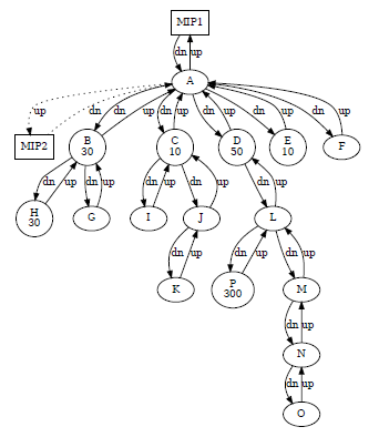
An simplified example of the particular structures (graphs) we have to deal with is provided in Figure 1, where a sub-graph for a target node L is shown. Suppose that an operator requests to allocate a band amount x over node L. From the whole graph, we have to extract or isolate the sub-graph in which node L is located including its neighbors and their (eventual) sub-trees in a recursive More precisely, staring from node L, we add nodes until: (a) a leaf node is found or (b) an END POINT node is found. We remind the reader that the ENDPoints set is given by the union of MIP and DC node sets (see Table 1). In order to simplify the plot even further, all links speed is set 1 Gbit/s and it is not shown explicitly.

Since we have a directed graph, each node can have in- bound and outbound edges which are respectively marked as down-link or up-link. Each connection between a pair of nodes it is actually implemented by a pair of edges: an up- link and a down-link edge. The route direction of up-link edges is towards an END POINT, while the route direction of down-links is towards leaf nodes.

Every node is enriched with its current reserved operator bandwidth (op_band) if it is ≠ 0. Note that current reserved

operator band parameter represents the cumulative amount of band reserved by any operator on that node. Dotted edges represents inactive links. This kind of edges usually connects a node A to one of the MIP nodes available. As depicted in Figure 1) node A is configured using an active-standby pattern, where the connection to MIP2 is the standby or back-up part which is exploited if and only if MIP1 link fails.

From Figure 1 it is intuitive to understand that the available bandwidth from node L have to take into account any consumption at any node in the sub-graph; in other words, each node that stem from any down-link sub-tree might contribute to bandwidth consumption and it must be taken into account.

The general idea is to manipulate the graph structure by enriching edges with a parameter (i.e., AvailBand) which keeps track of the current band availability measured in Mbit/s.

This annotated graph is suitable to calculate the residual band between any node ad its END POINT by running any well known algorithm [9, 10]. The algorithm is going to calculate the residual band on every edge in the sub-graph (by definition) and not just over the path between a target node and its END POINT.

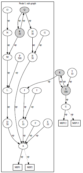
Unfortunately, real world conditions often present more complex scenarios. Figure 2 shows a prototypical, but realistic representation of a target node (L) sub-graph in our broadband network.

This sub-graph exhibits two main peculiarities: (i) it has two chain structures and (ii) two pairs of END POINT nodes. The former peculiar structure represents an exception to previous schema in which for any node pair (X, Y) we could only have one up-link and one down-link edge. Here, both edges are marked as up-links. This exception often allows the target node to reach multiple pairs of ENDPoints and this can complicate the band calculation as several (short- est) paths per END POINT becomes available. In addition, the larger the graph, the more challenging becomes its visualization and understanding.

In order to overcome these issues, we first need to clarify and impose that data traffic must follow the shortest path available to the closest END POINT and following the fastest links when possible. The closest MIP pair for a target node L is identified by the first steps of the algorithm. In the sub-graph, the set of nodes (LG) sharing the same closest MIP with target node L are the ones over which the actual band calculation is performed. In Figure 2, graph LG is the portion enclosed in the box.

More formally, we can express the available or residual band (RB) of node L in its sub-graph (i.e., see the box enclosed sub-graph shown in Figure 2) as:

$$RB(L) = \min\left(band\left(path_{L, \text{ENDPOINT}}\right)\right)\tag{1}$$

where the shortest path (path_(L,ENDPOINT)) is the smallest

set of edges {e_i,i+1, e_i+1,i+2, . . . , e_{i+(n−1),i+n}} connecting L to its END POINT. The band value for each e_{i, j} is the difference between the edge link physical bandwidth and the (total) operator band associated with the X_i-th node of the edge:

$$band(e_{i,j}) = phyband(e_{i,j}) – op\_band(X_i)\tag{2}$$

However, in order to address any operator band contribution from any node in the sub graph that may affect the edges over path_(L,ENDPOINT), we must consider all shortest paths starting from any node in the sub-graph having op_band ≠ 0. Essentially, in the case depicted by Figure 2, we have to consider the following set of paths and their corresponding band contribution over each edge:

$$\left\{ \begin{array}{l}
D \xrightarrow{50} A \xrightarrow{50} MIP_1 \\
P \xrightarrow{300} L \xrightarrow{300} D \xrightarrow{300} A \xrightarrow{300} MIP_1 \\
R \xrightarrow{10} M \xrightarrow{10} L \xrightarrow{10} D \xrightarrow{10} A \xrightarrow{10} MIP_1 \\
H \xrightarrow{30} B \xrightarrow{30} A \xrightarrow{30} MIP_1 \\
C \xrightarrow{10} A \xrightarrow{10} MIP_1 \\
E \xrightarrow{10} A \xrightarrow{10} MIP_1
\end{array} \right.$$

By summing all instances of the same edge e_{i, j} in the \((\textit{e.g., } D \xrightarrow{300} A + D \xrightarrow{10} A = 310~\text{Mbit})\) we obtain the total amount of band consumption over each edge. Essentially, we can rewrite (2) as:

$$band(e_{i,j}) = phyband(e_{i,j}) – \sum_{k \in I} (e_{i,j})_k\tag{3}$$

where I represents the set of instances, as visible in the previous schema, for each individual edge e_{i, j}. In (3), for any edge e_{i, j} we can actually calculate the (residual) band over an edge e_{i, j} by subtracting all op_band contributions from the physical bandwidth available on the edge link.

This approach [11, 12] allows us to calculate the available band for any target node in our broadband network no matter the complexity of the corresponding sub-graph.

3.1. Towards an ’holistic’ approach

After being able to estimate the residual operator bandwidth for a single node in the network, we started to focus our efforts in extending the calculation to the entire broadband network. In fact, in order to monitor our network health from a topological point of view, the fact of being able to check one node at a time quickly became too limiting.

Since our basic mechanism is capable of calculation the residual band for (any) node L and since each all sub-graphs adopted for the computation are not overlapping, extending the calculus over the whole graph2 sounds straightforward at least on paper. By adopting this approach, we can provide a global view of the bandwidth status of the broadband network and, by knowing which are the zones where band availability is suffering or barely sufficient, we can plan for an infrastructure upgrade.

Actually, we can move even forward.

Our tool, while searching paths over the graph structure can collect many interesting information. In particular, checking any topological issue is a natural consequence of visiting/searching over the graph. For example, we realized that the two following main issues are more common: (i) a path between two nodes is absent or (ii) a node from the sub-graph is absent. Especially the latter issue might stem from a mis-configured link property lying on the NMS which triggered a node removal from the sub-graph in one of the filtering phases.

In addition, we can build a timeline or history of the band allocation for any node and showing its evolution over time in terms of band allocation and infrastructure upgrades.

Finally, our goal is to enable the following three new features or sanity checks into Banda Calculus:

1. extract all critical path. A critical path is a path between any two nodes A and B where the available band is lower than a threshold band_tsd. We are interested in all critical paths according to the currently selected band threshold (band_tsd).
2. provide human readable information about any topo- logical issue eventually spotted by the algorithm while visiting the graph. The fact of having readable information is particularly important in order to simplify the task of fixing the (NMS) database, since it is carried out by a group of people.
3. build a time history about operator band for each node in order to be able to keep track of any change.

4. Algorithms

Our algorithm discussion is split into three distinct parts: the first one (a) is dedicated to the residual band calculation, the second one (b) is dedicated to the holistic sanity check features, while the latter (c) is about the graph visualization algorithm.

4.1. Bandwidth Algorithm

The basic idea underlying the algorithm in order to calcu- late the residual band for a single node is to first annotate the graph with an AvailBand parameter and calculating the bandwidth, as previously stated in Section 3. The annotation process requires several filtering steps over the graph which are aimed to ensure data consistency and normalization. These steps are summarized as follows:

• consistency check: it guarantees that each record in the JSON structure coming from the NMS API contains all parameters which are relevant for the band It ensures that their values are in their corresponding ranges and are not null or NaN. A graph object G is generated at the end of this step.
• first filtering: from the previous polished graph G it is extracted a sub-graph SG according top a selected target node L. The graph SG is identified through a Breadth-First Search (BFS) over G starting from node L. The search stops when an END POINT or a leaf node is found.
• second filtering: SG sub-graph is refined a second time in order to just select only the relevant edges. More precisely, only edges with the following characteristics are kept:
  • edge parameter is_active is true
  • edge parameter template is not “NA”
  • edge parameter dir is “uplink”

During this step, each edge is annotated with an AvailBand which is initialized to the current edge speed parameter value.

• third filtering: finally, graph SG is further reduced in case multiple ENDPoints are present. According to the chosen target node L, its closest MIP (or MIP pair) is selected (i.e., MIP_closest) and all nodes sharing MIP_closest as their closest END POINT are kept in SG.

This third filtering is only applied when the actual band calculation is triggered.

The requirement to address each allocation contribution provided by nodes in any graph sub-tree as well as in chain structures, forces the algorithm to consider all shortest paths from every node to the MIP and not just from leaf nodes.

Figure 3 shows the calculation algorithm using a pseudo- code notation. The code does not take into account the consistency check filter. It is basically split into three parts. The first one is dedicated to the filtering processes (i.e., lines 1-9).

The second one (i.e., lines 10-14) computes all shortest paths between every node and the sub-graph ENDPoints. paths is a map or dictionary structure which collects the path set for each node. The latter part instead (i.e., lines 15-28) perform the actual graph visit and updates the AvailBand field over each visited edge. During the visit, any node having allocated bandwidth – op_band field > 0 – and being still unknown, becomes part of the already known nodes in order to guarantee an exactly once semantic of the algorithm.

4.2. Sanity check algorithm

The sanity checks algorithm, expressed in a pseudo-code notation, is depicted in Figure 4. The idea is simple and its actuation is scheduled at regular intervals (i.e., ∆=24 hours). For each node in the main graph (component) G we call the main function (get_banda()) which is the one depicted in Fig- ure 3) which provides specific data structures required for our application needs. More precisely, it works as follows. The initialization phase (e.g, lines 1-4) prepares several data object, such as a set for basic nodes (i.e, no ENDPoints), a set for collecting topological issues and a database handle where the band history is actually stored.

The procedure runs until the node set is not empty (e.g., line 5). Nodes are pulled from the set one at a time in a (uni- formly) random order and the residual band is calculated on the selection (e.g., lines 6,7). The get_banda() function invocation generates two structures: (a) a banda_path object holding the path from a target node to its MIP and the corresponding residual band and (b) a subG object which represents the target node sub-graph with nodes and edges enriched. Nodes are annotated with their allocated opera- tor band, while edges are annotated with their respective residual band values.

At line 8, nodes belonging to the current target node sub-graph are removed from the node set since the band is computed for all nodes in the sub-graph. Any eventual node band update is propagated on stable storage over the database (e.g., line 9).

Finally (e.g., lines 11, 12), in case of exception, a handler manages any arising error. Three kinds of exceptions are actually trapped, which are the following:

• NoPathException: no path is found between node A and B, where B is a MIP. This exception may arise when there is a missing up-link edge between the two nodes. Actually, it is likely due to a mis-configuration in the NMS: in fact the edge can be present but it might have a wrong label, such as configured as ’down-link’ instead of ’up-link’.
• NoNodeFoundException: a target node A or the MIP B is not found in the The reason for this exception is likely due to the removal of this node during one of the filtering processes. Again it is likely due to a NMS bad configuration: in fact a node might has been removed from the graph if all its edges are marked as ’down-link’.

1 G ← 1st_filtering()

2 G ← 2nd_filtering()

3 nodes ← G.nodes()       ENDPoints

4 avail_mips ← G.sample()

5 known ← SET()

6 if avail_mips.length > 2 then

7              G.filter_closest_mip(target_node)

8              avail_mips ← G.sample()

9 end

10 foreach node ∈ nodes do

11             foreach mip ∈ avail_mips do

12                       paths[node] ← G.dijkstra(node,mip,weight=SPEED)

13             end

14 end

15 foreach node ∈ paths do

16             used_band ← 0.0

17             path ← paths[node]

18             source ← node

19             foreach item ∈ path do

20                       cur_band ← G[source][item][AVAIL_BAND]

21                       if G.nodes[source][OP_BAND] > 0.0 ∧ source g known then

22                                 used_band ← used_band + G.nodes[source][OP_BAND]

23                                 known ← source

24                       end

25                       G[source][item][AVAIL_BAND] ← cur_band – used_band

26                       source ← item

27             end

28 end

Figure 3: Residual band algorithm pseudo code.

• BadLinkException: in this case the system cannot calculate any path since there are no ENDPoints available in the sub-graph. Here, it is very likely that the sub- graph MIPis connected through ’inactive’ edges and this triggered its removal from the Again, the underlying reason is a badly configured NMS.

4.3. Visualization Algorithm

It is important to note that this algorithm just focuses on graph visualization and it does not affect the band calculation in any manner. While the graph objects we manage are not huge, their size is in a range that poses a challenge when trying to display them into a graphic interface window. In fact, it is not unusual to deal with a node whose sub-graph is about 1000 nodes in size. This especially happens when radio bridge (i.e., PR) nodes are involved: since all their edges are marked as uplink, they are likely to join distinct parts (sub-graphs) of the broadband network by creating loops that are not filtered out by the standard processing that is performed.

Even a few hundreds nodes and their edges end up in chaotic plot when trying to display them. In addition, this plotting effort is quite useless because it is likely that the vast majority of the (sub) graph does not participate to the bandwidth consumption: only the set of nodes having the same closest MIP as the target node are actually involved. We remind the reader that the third filtering step is only applied when the actual band calculation takes place. There- fore, the sub-graph is not simplified yet. However, even if the sub-graph would have been simplified at this time, it might be too large as well to obtain a non chaotic plot.

In any case, when dealing with such oversize sub-graphs we need to make a decision and choosing what we are really interested to. It is not a matter to choose or design a new plotting layout. When a user have to check the residual band for a target, the goal is to see the situation over the path that links the target node to its ENDPoints. The more we move far from this path, the less is the interest and the value for the information.

The amount of available band along this path is of course dependent by the eventual contribution coming from any sub-branch at each path node, but these contributions are calculated by the previous algorithm (see: 4.1) and affect the band availability at each edge.

According to what we just stated, the basic idea underlying the visualization algorithm is to first focus on the shortest path connecting the target node to its closest MIP (i.e., or 

1 repeat periodically every ∆ time units                                                                                 % Code executed every ∆=24 hours

2              nodes ← G.nodes()       ENDPoints

3              G_errors ← ∅

4              history ← DB.instance()

5              while nodes ≠ ∅ do

6                        node ← nodes.sample(1)

7                        banda_path, subG ← get_banda(G, node)

8                        nodes.pop(subG.nodes())

9                        history.update(node, banda_path, subG)

10             end

11             on GraphException : ex do

12                       G_errors ← ⟨ ex.node, ex.info ⟩

13             end

14 end

Figure 4: Algorithm pseudo code for sanity checks calculation.

1 K_MAX ← 50;                                        % Constant: max number of nodes for visualization graph

2 avail_mips ← G.getMips()

3 mip ← avail_mips[0]

4 path ← G.dijkstra(target_node, mip, weight=SPEED)

5 simple_G ← G.subgraph(path).copy()

6 foreach item ∈ path and simple_G.size() ≤ K_MAX do

7              if not item.isMIP() then

8                        extra_nodes ← G.subgraph([G.allNeighbors(item) + item]).copy()

9                        simple_g ← compose(simple_g, extra_nodes, K_MAX)

10             end

11 end

Figure 5: Banda Calculus Algorithm pseudo code for generating the simplified graph suitable for visualization.

MIP pair), then to expand this “graph-path” by adding the neighbors of each node belonging to the shortest path. Any i+1 level of nodes can be added by iterating the last step over the previous level of added neighbors. As a general rule, this process can stop when the graph size reaches K_MAX (e.g., with K_MAX=50).

In such a manner, we can plot what it is really required.

The actual algorithm pseudo code is depicted in Figure

The first four lines are in charge to detect the MIP nodes in the target node sub-graph (e.g., which is G in the code). Shortest paths are calculated using Dijkstra algorithm and a simple_G graph object is This graph just contains the path items, the original sub-graph MIPs and their arcs.

The simple_G object is enriched by adding all neighbors for each node member of the shortest path (i.e., see lines 5-10). Any member being a MIP is skipped. The graph size is limited by the constant K_MAX both in the loop statement and by the commodity function compose() which actually merges two graphs together. More precisely, these graphs are: (i) the simple_G object and (ii) the graph made by the current loop node (i.e. item) and its neighborhood (i.e., see line 8). Any node or arc is added just once.

5. Implementation

Banda Calculus is implemented in Python3 language and through the adoption of other several frameworks for specific tasks.

Actually, the evolution of Banda Calculus leaded to several implementation over time since 2019 [11]. At first, it was designed as a Jupyter [13] notebook. This choice is quite common in the data science area and it turned out to be rewarding for our goal as well.

When started, this work shared many similarities with data science projects, where data sets have to be understood, analyzed and verified. For this reason, Jupyter turned out to be a stand out candidate for prototyping our tool. Usually, the best practice working with Jupyter involves trying ideas and distilling a corpus of functions or classes and use them as basic building blocks, then this process is iterated until the problem is solved.

By following this practice, we first designed the Banda Calculus application as a Jupyter notebook by exploiting exploits the set of modules we distilled. By mixing code and code and formatted text elements, a notebook can simplify documentation management. The notebook implementation helps the user in how to install a Python virtual environment and the required project dependencies. In addition, the built-in documentation provides a user with a step by step explanation of (i) what he is supposed to do in order to use the tool and (ii) how it works.

Among the several solutions to manage a graph structure in Python, we selected NetworkX[14] library. The main reasons is that it is strongly supported by the Open Source community, it has a wide collection of state-of-the-art grade graph algorithms, and it is symbol oriented; in other words, any element identifier of a graph can be a symbol (e.g., a string or any complex object instead of a numeric id) and this simplifies data management. Symbolic graph libraries are not as fast as lower level ones, but the graph we are working with are in a manageable range (e.g., ∼3550 nodes and ∼8100 edges).

For visualizing graphs inside a notebook we adopted frameworks (e.g., Holoviews and Panel) taken from the data science world. These are high level frameworks suited for large data-sets.

Figure 6 shows the output of Banda Calculus notebook application. It performs the following logical activities:

• Graph creation: the application downloads a graph structure using the API and stores the corresponding graph object on stable storage labeling the file with the current date in graphml However, if the current date matches the one of any available graph file, then this file is loaded instead. When the API fails for any issue, the most recent available file is loaded.
• Target node selection: through a Graphic User Interface (GUI) widget the user can select the desired target node from a drop-down list containing all valid nodes found in the This choice is recorded and remains set for the entire notebook.
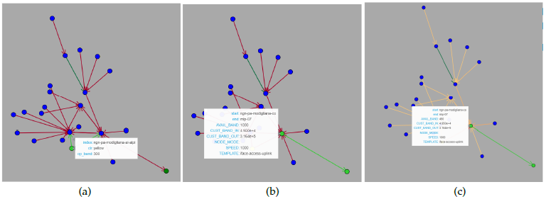
• Sub-graph initialization and visualization: graph initial- ization and its visualization are split in two distinct notebook cells. The output of the latter is depicted in Figure 6. The first two plots (see Figure 6(a) and (b)) are respectively dedicated to the visualization of nodes and edges attributes.

The item color code is the following: target node is yellow, ENDPoints are green and standard nodes are blue. The edge color scheme instead is given by a (linear) color gradient function based on the corre- sponding speed field: faster edges are towards green, while slower ones are towards red. Any part of the sub-graph can be inspected by dragging any element or zooming. Due to their average length, node names are only visualized when moving the cursor close to their shape. By exploiting this visualization the user can check the current op_band allocation and the edges speed field.

• Operator band calculation and visualization: the sub-plot in Figure 6(c) shows the target node sub-graph after the residual band calculation. As sub-plot (b), this visualization is edge By inspecting the edge (i.e.: linking: ’ngn-pa-modigliana-co’ → ’mip-07’) we can see the AvailBand field annotated with the actual residual bandwidth. From the GUI it is possible to follow any path and inspecting the bandwidth at each hop. In addition, the output cell of the notebook shows bandwidth information along the path between the target node and its END POINT:

ngn-pa-modigliana-ai-alpi –[a. band: 700.00 Mbit/s]->
ngn-pa-modigliana-co
ngn-pa-modigliana-co –[a. band: 460.00 Mbit/s]-> mip-07

One of the notebook features we believe is very beneficial for our goal is the possibility to convert it into a standalone web application in a straightforward manner.

For example, this would open the road to deploy our tool in a container and serving users on the one with a traditional server approach.

Unfortunately, while the notebook app is up to the task of calculating the residual band and by exploiting the adopted frameworks it is possible to obtain a working web applica- tion with zero effort, the GUI offered by the notebook is too limiting and the documentation provided by the notebook itself is still too technical for non-tech users. Expanding and adding more sophisticated features to the notebook app is likely to became quite challenging. For this reason, we

decided to refactor our design and to switch to a different implementation capable of providing a full web application.

5.1. Web Implementation

Our implementation of the web version of the application and its ’holistic’ features for network sanity checks is still grounded on Python3, but the adoption of another frame- work – Plotly-Dash [15] – is responsible of enabling the web interface without requiring any knowledge of standard web technologies (e.g., Javascript or CSS). Surprisingly, we man- aged to keep Jupyter in our design pipeline since Plotly-Dash is compatible with it and a single statement is just required to switch the application from running inside Jupyter to running standalone.

In other words, our approach of prototyping the basic functionalities into a Jupyter notebook [13] still holds.

Other frameworks has been adopted and are responsi- ble for specific tasks such as Cytoscape [16] for rendering graphs on a web interface.

The new feature of keeping track of node band allocation over time requires some kind of database storage. Both a relational or NO-SQL approach are suitable and we decided to go for the traditional (relational) approach. In particular, we just adopted a SQL interface provided by the SQLite package and not a full database system. In fact, at the time of writing, the amount of stored data does not deserve a more sophisticated solution. However, this is likely going to change in the near future in order to improve the robustness and flexibility of the system. Since the application runs in a

Docker container in our production environment, adding a database system is straightforward. Two persistent volumes has been added to the container to preserve data on stable storage which are respectively dedicated to: (a) database file and (b) daily graph files.

All sanity checks discussed in Section 3.1 are computed (once a day) when the application downloads the raw net- work data from the NMS API and builds an updated graph structure. Both sanity checks and the download procedure run inside a background service written in 100% Python as well. The web app exhibits the same behavior as in the previous implementation (see Section 5).

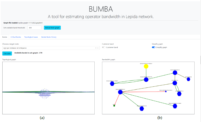
Figure 7 shows our tool GUI dedicated to the residual bandwidth calculation of a specific, single target node. In fact, note that the GUI has a first tab labeled as: “Banda” activated. The application GUI has been refreshed to better integrate the new features related to graph health.

The button labeled “Reload fresh graph” on the web Graphical User Interface (GUI) manually triggers the load of the freshest available graph from local storage. This tab performs the same task as the previous notebook application with some usability improvements.

After choosing a target node from the drop-down widget labeled “Choose a target node“, the corresponding sub-graph is rendered in the “Topological graph” widget window. After applying the filtering process (until the second filter, see Section 4), the graph is still too large and its rendering provides little help to the user trying to visually verify the sub-graph topology. In these cases, enabling the switch labeled “Simplify graph” substantially simplifies the graph rendering and allows users to concentrate over the interesting part of the sub-graph. After enabling the switch, by pressing the Calculate button the bandwidth calculation is performed and this triggers to effects: (i) the amount of available bandwidth appears close to the button and (ii) the simplified graph is rendered on the Bandwidth graph window. By enabling the simplified rendering before choosing the target node, it would have also simplified the rendering for the Topological graph. Here, only the graph on the right is simplified because the switch has been enabled after the target node selection.

In graph renderings, all nodes have a rounded shape except MIP nodes, which are squared and green. Target nodes instead are yellow and any other node is blue. When graph simplification is enabled (see ’Simplify graph’ switch widget in Figure 7), border nodes are rendered in a hexagonal shape. Border nodes are neighbors of any node being part of the shortest path starting from the selected target node. Node size is dynamic and changes according to a linear function applied to its op_band value.

The edge color meaning varies according to the particu- lar graph window. In the topological graph widget (i.e. the left widget), the edge color represents the link speed: faster links are green, while slower links tends towards red. In the bandwidth graph widget instead (i.e., the right widget), the edge color shows the calculated residual band over that link. Its color scheme is the same as in the previous widget. Any edge connecting to a MIP node in standby mode is represented as a black dashed line and labeled by a red “standby” text on top.

Also in this application version, graph plots are dynamic and each element can be dragged and zoomed.

In addiiton to the “Banda” tab, this version has been enriched by three other tabs which respectively correspond to the graph sanity check features. The new tabs are named as follows: “Critical Banda”, “Topological Issues” and “Banda Node History”. In the following, we are going to focus on their respective interfaces.

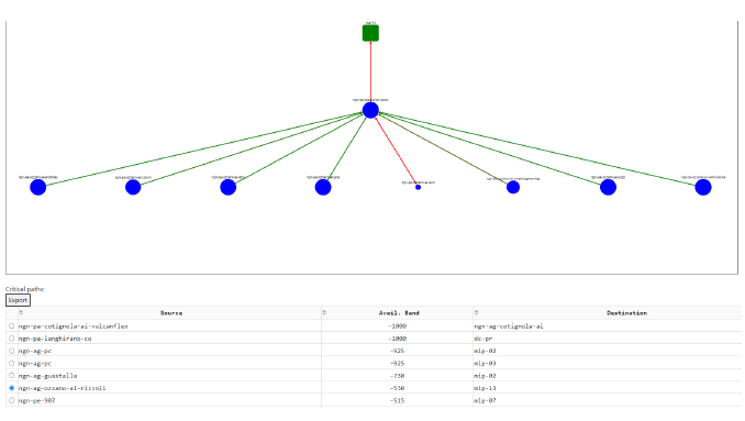
The “Critical Banda” tab interface is shown in Figure 8. The graph plot shows the topology of a sub-graph which is the one in which lies the selected edge picked from the bottom table. The plot edges color shows their status. In fact, the selected edge is represented in red color as well as “ngn-pa-ozzano-ai-iaco” → “mip-13” edge.

The threshold that defines a critical link is towards the top of the GUI page and it stays visible no matter which tab is selected (see 7). The threshold (band_tsd) default is set to 300Mbit/s and can be overridden by editing its widget. Any edge whose residual band is less than the threshold is collected into the bottom table.

The table content can exported (in CSV format) through the “Export” button on the table top left corner.

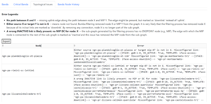
The next tab is dedicated to topological issues and it is shown in Figure 9. Here, a table collects any exception error triggered by search algorithm over the graph (i.e., G_errors data structure). For each target node triggering an exception we have a table record with a corresponding “Node” column. The “Error” column contains all the required information (such as: node names, device interfaces, template description, . . . ) in a human readable form in order to fix the corresponding issue on the NMS. As in the previous tab, the table data can be downloaded for offline processing through the “Export” button.

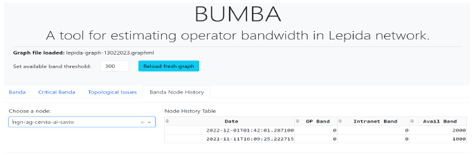
Figure 10 shows the tab dedicated to node history. A user, by choosing a target node through the left drop-down widget, can query the underlying knowledge-base about any bandwidth allocation change over time. The node selection triggers the visualization of the corresponding information by populating the table on the right.

These new features allows to obtain an overview of the bandwidth status of the whole network graph and they fo- cus on emphasizing those elements that are likely to deserve a special attention.

5.2. Banda Calculus API Integration

In order to support and integrate with other Company services, Banda Calculus implements a basic REST API in order to allow systems to interact together without human intervention. The API exposes a single resource via GET HTTP method. It is just sufficient to specify the target node symbol name as the only parameter. The back-end system reply is represented by a JSON structure as follows:

{
’target_node’: <node_name>,
’avail_band’: <band-int>,
’path_to_mip’: [(<node-A>, <node-B>, <band-int>), …, ()],
’from_graphfile’: <graph_filename.graphml>,
’message’: ’OK’
}

The object contains the target node symbol provided as parameter and the field avail_band shows the final re- sult of the banda calculation process towards the closest MIP. In path_to_MIP field, a list of tuples depicts the exact path followed by the algorithm and specifies the residual band for each edge. Other information, such as the specific graphml file adopted as data source (i.e., from_graphfile) and a human readable outcome message (i.e., message). The former field contains the string ’OK’ or an error string in case of any issue.

6. Discussion and Conclusions

In this paper, we presented the problem we tackled when dealing with checking residual bandwidth availability in our Regional broadband network. Our ad-hoc and in house- developed solution, Banda Calculus, is coming from this particular need. Since the very beginning, the main benefit introduced by our tool is the substantial reduction (e.g., seconds versus hours) of the time required to calculate the residual available bandwidth over a specific node. Just this step turned out to be a game changer in order to provide our services to customers.

The benefits introduced by Banda Calculus are not lim- ited to getting faster, streamlined business procedures. In fact, its evolution over time introduced several features ad- dressing other needs. It first evolved in terms of (a) usability by becoming a web application deployed in our Intranet and in terms of (b) focusing on the whole network instead of a single node at a time. In particular, the latter avenue of evolution expanded the range of features at our disposal. These

features improve our monitoring and planning capabilities. We briefly summarize them in the following lines.

By exploiting the health monitoring features, operators can understand (c) in advance which parts of the (sub)graph might need un upgrade before it is too late (e.g., unable to provide any bandwidth). In addition, anything which is suspected of being a topological graph issue (d) is reported in a table and it is open to inspection. Also the graph visu- alization has been fine tuned and we adopted an in-house developed algorithm (e) that can be triggered when dealing with large graphs. Finally, in order to integrate Banda Cal- culus into our company processes and to allow automatic interactions between systems, we provided an API (f).

Our near future plans are actually focused on integration in order to automate and integrate as much as possible our business processes.

1. “LepidaScpA Home Page”, 2022.
2. “Nagios Monitoring Solutions”, 2022.
3. “Network monitoring with intuition”, 2022.
4. V. J. Ribeiro, J. Navrátil, R. H. Riedi, R. Baraniuk, L. Cottrell, “pathchirp: Efficient available bandwidth estimation for network paths”, 2003.
5. R. L. Carter, M. E. Crovella, “Measuring bottleneck link speed in packet-switched networks”, Performance Evaluation, vol. 27-28, pp. 297–318, 1996, doi:https://doi.org/10.1016/S0166-5316(96)90032-2.
6. M. Allman, “Measuring end-to-end bulk transfer capacity”, “Proceed- ings of the 1st ACM SIGCOMM Workshop on Internet Measurement”, IMW ’01, p. 139–143, Association for Computing Machinery, New York, NY, USA, 2001, doi:10.1145/505202.505220.
7. “Elastic Stack”, 2022.
8. “Graphana Labs”, 2022.
9. “NEO4J Graph Data Platform”, 2022.
10. Y. Dinitz, Dinitz’ Algorithm: The Original Version and Even’s Version, pp. 218–240, Springer Berlin Heidelberg, Berlin, Heidelberg, 2006, doi:10.1007/11685654_10.
11. Y. Boykov, V. Kolmogorov, “An experimental comparison of min- cut/max-flow algorithms for energy minimization in vision”, “Thirdy Minimization Methods in Common and Pattern Recognition”, vol. 23, pp. 1124–1137, 2004.
12. G. P. Jesi, G. Mazzini, “Banda calculus: a tool for bandwidth estimation in broadband network infrastructures”, “2020 International Conference on Software, Telecommunications and Computer Networks (Soft- COM)”, pp. 1–5, 2020, doi:10.23919/SoftCOM50211.2020.9238312.
13. G. P. Jesi, A. Odorizzi, G. Mazzini, “Exploit company knowledge from graphs with banda calculus”, “2021 International Conference on Software, Telecommunications and Computer Networks (SoftCOM)”, pp. 1–6, 2021, doi:10.23919/SoftCOM52868.2021.9559101.
14. “Project Jupyter”, 2022.
15. “NetworkX – Network Analysis in Python”, 2022.
16. “Low-Code Data Apps”, 2022.
17. Cytoscape – Network Data Integration, Analysis, and Visualization a Box”, 2022.

Citations by Dimensions

Citations by PlumX

Crossref Citations

This paper is currently not cited.

No. of Downloads per Month

No. of Downloads per Country