Neural Network regression (NNR) is considered more effective as compared to multiple neural networks model readily available in Azure to evaluate the Remaining Useful Life (RUL) of bearing in this work because it performs better than other models when used and was demonstrated as a non-programing technique for analyzing enormous data without the use of Hive, Hadoop, Pig, etc. To complement the earlier paper, we further used statistical means in verifying our results. Using this non-parametric non-linear approach is intuitively appealing to forecast the Remaining Useful Life (RUL) of a bearing. Over the years the Azure cloud service platform has gained recognition as a major forecasting technique toolbox of forecasters, NNR model implementations have surged, hence its inclusion here on its’ use on the NASA FEMTO-ST Institute (Franche-Comté ÉlectroniqueMécaniqueThermique et Optique – Sciences et Technologies) bearing dataset. Azure is a machine learning platform from Microsoft that allows developers to write, test, and deploy algorithms and has been motivationally proven adequate and useful for predicting the RUL of bearings. As seen in so many recent articles, NNR Artificial Intelligence is a model among many others readily available for computing on the platform that has been successfully used for non-programming of the enormous dataset and applied for forecasting the RUL of Bearing. This has added value in the forecasting phase. The novelty in this work is related to the application of NNR where we were able to combine the Dickey-Fuller Test with NNR to ensure that the data needed to be used with NNR is fit for application to yield optimal prediction results and our previous result from the past paper was further established. A satisfactory judgmental result was obtained; making Azure's work studio a reasonable place to predict without much programming expertise. We tested the findings from the National Aeronautics and Space Administration (NASA) database for the person that came first in the competition by comparing our Azure model observations with the NNR observations collected. Ultimately, we showed the finding is enhanced by the AZURE model.

1. Introduction

This paper is an extension of work originally presented in [1], which involves the prediction of the remaining useful life of bearings thereby checking to see if the normal big dataset could be structured and analyzed by using the models found on the Azure machine learning platform which are meant for cloud computing. This was found to be of major relevance in the field of condition-based maintenance. Lots have been said about artificial neural capabilities learning and popular networks in recent articles. Non-linear regression is often widely used for non-linear systems. However, there is a need to combine the use of statistical models with non-linear data for better prediction performance. Here in this research work, attention is paid more to cloud computing models application with a special focus on Azure virtual machine which was used in the previous conference paper to corroborate our results from our previous work. Neural networks are composed of a broad class of non-linear functional regression and non-linear data analytic models. They also consist of a large number of “Neurons,” (referring to the basic linear or non-linear computing elements) well connected by means that are often nuanced and organized into layers [2, 3].

Azure is a popular cloud service powered by Microsoft and there are other popular cloud services also readily available. Concerning Azure cloud service, this is accessible in 60+ geographical regions, with well over 200 accessibility areas. It offers a robust portfolio of Infrastructure as a Service (IaaS), as well as powerful features of Platform as a Service (PaaS), especially for Windows applications. You can make your applications immune to failure or interruption in your primary data center by running the services on multiple availability zones.

Using a wide class of non-linear complex systems the neural network (NN) is a powerful building tool particularly in the application of control strategy when considering features such as inputs, variable system states, and control behavior such as the output of the system, which is found to be paramount in systems. The open and closed loop control feedback identification is two classes of control application [4]. Some areas of application are found in sonar detection, translation of English text into phonemes, machine vision, forecasting in economics, and marketing of airline seats as well as in the banking sector. Most of these applications require pattern recognition, this is because the pattern recognition problem is parallel which involves the processing of several different pieces of information that all tend to interact with one another to create a solution [5]. However, identifying the basic problem with control closed-loop feedback in NN is the provision of an online learning algorithm which more often does not require off-line initial training that involves the simulation of complex non-linear functions.

Artificial intelligence is an extremely valuable method in non-linear systems [6]. This implies that when designing a hybrid control system, a model-based controller might be suitable to replace the intelligent control systems for systems having mixed conventional approaches.

The ability to manage large data sets rapidly and to operate them parallel to input variables has rendered neural networks versatile when it comes to their application. Artificial Neural Networks offer a favorable substitute method in forecasting. The neural network’s non-linear innate structure has readily contributed to its usefulness for taking the dynamic causal relationship in many real-world problems. Forecasting applications have been rendered more flexible because Neural Networks (NN) not only made it possible to identify the non-linear structures in a problem, they also make modeling linear processes easy as well [7- 9].

In [10] Neural Network was applied in tracking machine-driven defects of rotating parts. Their work contribution involves the application of preceding values of data, as being inputted into a system for the prediction of patterns. They also believed that the amplitude of vibration could show the machine’s progressive deterioration among other parameters. This rate of increase is proportional to the severity of destruction/damage. In this work, we were able to relate the application of NNR with Dickey-Fuller Test to yield an optimal prediction result which was initially covered in a previous conference paper to which this serves as an extended work.  However, the limitation(s) of this study lies in the inability of the authors to further generate more data to validate their results due to proxy reasons. For suggestions of direction for future work, we will advise also the inclusion of axial loading to the radial loading done on the bearings for better real-life failure capturing. In section 2.0, the model analysis theory about NNR was covered. The background to Neural Networks Regression was also covered in section 3.0 and in section 4.0 the experimental work involved was discussed. Section 5.0 and 6.0 relates to the results and discussion, and conclusion respectively.

2. Model Analysis for Condition Base Maintenance

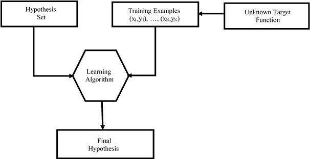
Machine learning could be said to be an advanced application of the statistical model with the help of machines. Fault diagnosis has been achieved in a model-based diagnostic system by comparing the model design system with the system’s actual monitored condition. Diagnostic and prognostic analytics is a data-driven approach that is suitable for condition monitoring. The data-driven diagnostic and prognostic methods are often analyzed with statistical tools, AI, and other approaches. Model-based diagnostic (MBD) infers to an artificial intelligence area of fault diagnosis. Figure 1, gives a sketch of the processes involved with the learning model.

Often based on mathematical models is the model-based approach that is needed to epitomize the behavior of the system, about the phenomenon of degradation. Physical models are very much useful in the accounting field for all operating conditions. However, statistical models are established from the input/output data collected, which excludes unrecorded circumstances. Approaches that are close to model-based techniques work unswervingly on signal data without using mathematical models, this method adopts the signal processing techniques to identify signal data patterns/signatures.

In industrial applications, collecting reliable data for use in a data-driven model is more stress-free than constructing physical models, which gives the upper edge for data-driven models over physics-based prognostic approaches, whereas generating behavioral models (data-driven) from real-condition data leads to having predictive results which are more accurate than those of the physical model [11, 12].

In general, acoustic and vibration sensor signals are measured to determine the condition of the bearings and compared with the reference measured signals. Industries usually diagnose damage progression in the life cycle from a very early point, so tracking the health condition of mechanical low-speed and heavy-duty systems is of great importance. The interpretation of signals from condition monitoring can be done by various methods, including time-domain analysis, frequency-domain analysis, and time-frequency analysis. The frequency domain analysis is the most often used transformation technique because of the Fourier transforms simplicity of operation and its ease of interpretation [13].

3. Theoretical Background of Neural Networks

Neural Network analysis is paramount to this work as it includes an extension of the Neural Network. Therefore, their biological origins, possible applications, and their various architectures will be briefly discussed.

The NNR model which presently is one of the best for data analysis is a method for evaluating the relative significance of a combination of inputs to predict a given outcome. Usually, the model class is composed of layers of elementary processing units, known as nodes or neurons, which use a non-linear transfer method/function.

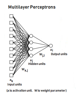
Figure 2, displays the learning model for a neural feed-forward network. They are most often multilayer perceptron in a structure consisting of input nodes that are connected by weights to hidden units or nodes. Depending on how complex the structure is, the hidden layer architecture may be of so many layers in the structure consisting of several nodes. Finally, the last stage of the hidden layer feeds the outer layer/node(s) [14].

A simple perceptron calculates a linear input combination (often with an interceptor bias term) which is called net input. Generating the output often involves a likely non-linear activation function. An activation function maps every real input into a relatively small range, often between -1 and 1 or between 0 and 1. Bounded activation functions are also referred to as squashes. Some common enabling features are presented below:

• Hyperbolic tangent: act(x)=tanh(x)
• Linear or identity: act(x)=x
• Threshold: \(act(x) = 0 \ \text{if} \ x < 0, \ 1 \ \text{otherwise}\)
• Logistic: \(act(x) = (1 + e^{-x})^{-1}\)
• Gaussian: \(act(x) = e^{-x^2 / 2}\)

Differing the number of hidden layers and the number of hidden neurons in each hidden layer will vary the complexity of the multilayer perceptron (MLP) model. An MLP is a parametric model with a small number of hidden neurons which provides a useful alternative to polynomial regression. MLPs are general-purpose, modular, non-linear models which can approximate virtually any function to any desired degree of accuracy, provided enough hidden neurons and sufficient data are given to it. To put it in another way, MLPs are universal approximators [15]. Figure 3, lists the typical symbols used for the neurons.

Therefore, in the vector of variables, we need to find the local optimum by the gradient methods for minimizing the function \(\hat{L}(\vec{W})\) range (W range). It is necessary to remember that, in this case, the \(\hat{L}\) function rest on constant standards 𝑥⃗ which represent the perceptron inputs. The \(\hat{L}\) function in eq 4 relies on h which is non-convex, so it is not possible to solve the optimization problem simply by resolving some ∇\(\hat{L}(\vec{W})\) =0. The complete input node 𝑥_𝑗 is formally known to be the point product between the weight vector 𝑊_𝑗, and the input vector A subtracting the weighted bias data. The output value of the resulting processing unit 𝑥_𝑗 then passes via the non-linear transfer function [16].

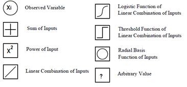
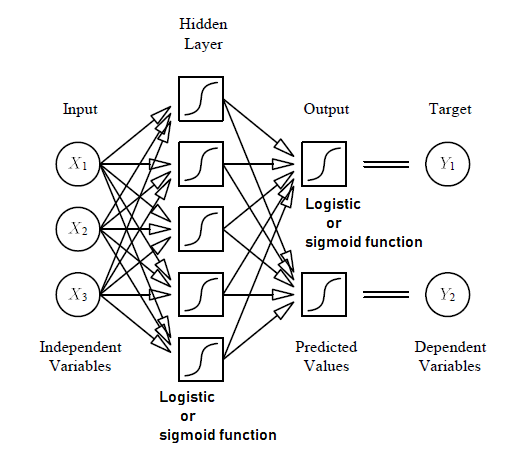
Figure 4, demonstrates a multivariable non-linear deep neural network regression. Consider a multilayer perceptron (MLP) with three input nodes, two output nodes, and a hidden layer with logistic or sigmoid activation function to match a basic non-linear regression curve as shown in Figure 4. Many wiggles may be in the curve as there are hidden neurons (actually there may be even more wiggles than the number of hidden neurons, but its estimation appears to become more difficult in that case). This basic MLP works more like a smoothing spline or least-squares of the polynomial regression. The Regression or response function f describes the effect of independent variables on the answer mathematically [9, 16].

$$y = f(x_1, x_2, \ldots, x_n, \beta_1, \beta_2, \ldots, \beta_n) \tag{1}$$

where y is the dependent variable

𝑥₁, 𝑥₂, ……., 𝑥_𝑛 are the input variables

𝛽₁, 𝛽₂, ……, 𝛽_𝑛 are the regression parameter not known and 𝑓 is the function usually assumed to be known.

The regression model for the response variable as observed is written as:

$$z = y + \varepsilon = f(x_1, x_2, \ldots, x_n, \beta_1, \beta_2, \ldots, \beta_m) + \varepsilon \tag{2}$$

where ε is the observed error in z

The unknown regression parameter {𝛽₁, 𝛽₂, ……, 𝛽_𝑚} can be determined by the method of least squares

$$E\{\beta_1, \beta_2, \ldots, \beta_m\} = \sum_{j=1}^{n} \left(z_j – y_j\right)^2 = \sum_{j=1}^{n} \left(z_j – f(x_1, x_2, \ldots, x_n, \beta_1, \beta_2, \ldots, \beta_m)\right)^2 \tag{3}$$

where 𝐸{𝛽₁, 𝛽₂, ……, 𝛽_𝑚} is the error function or the sum of squares of the deviations.

To estimate 𝛽₁, 𝛽₂, ……, 𝛽_𝑚 we minimize 𝐸 by solving the systems of equations

$$\frac{dE}{d\beta_i} = 0, \quad i = 1, 2, \ldots, m$$

When learning the model the weights on the training set help to minimize the errors. The square error with 𝑥⃗ and Y is given by the following equation

$$L = \frac{1}{2} \left( Y – h(\vec{W}, \vec{x}) \right)^2 \tag{4}$$

The pseudo-code for the algorithm on the process of obtaining the remaining useful life of the bearing base on the use of the NNR model is presented below. This algorithm is quite explicit enough except for instruction 1 which entails the application of corrective measures when the data fitness condition is not met. However, a brief expository is presented here on it. There is often the need to perform a data fitness test on the collected data to ascertain if the data is stationary data or non-stationary data. This usually involves the use of statistical tools and the performance of differential functions on the dataset to ensure that the data is non-stationary or non-linear before its application if found stationary.

4. Experimental Procedure

PRONOSTIA is a research rig device (Figure 5) used primarily for inspecting and validating the identification, diagnosis, and prognosis of bearing failures. An AS2 M team from the FEMTO-ST Institute designed and built the platform.

The PRONOSTIA aims to provide experimental proof in real-time, thus characterizing the deterioration of the ball bearings during their working life (it is still experiencing total failure) [17]. The PRONOSTIA data provided from the platform is unique being that it corresponds to the normal degraded bearing. The test rig allows us to perform the degradation of the bearings in just a few hours.

The defects are not artificially placed on the bearings, and all types of defects (balls, rings, and cages) are said to compose each damaged bearing. Constant operating conditions that include the data provided for each experiment performed on the PRONOSTIA test rig generates data on bearings that are degraded under unfavorable operating conditions.

There are three main parts that the test rig platform is made of; a part of rotating components, a generating part causing deterioration, and a part of the measurement.

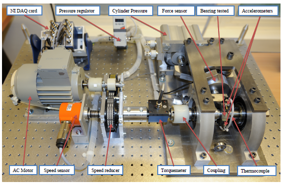
A power equal to 250W is transmitted via the spinning motion of the rotating motor through a gearbox, allowing it to generate a secondary shaft speed while retaining its rated torque at speeds below 2000 rpm, thus enabling the motor’s maximum speed to reach 2830 rpm. The radial force reduces the life of the bearing by restricting the total dynamic charge of the bearing to 4000 N. Details of the loading parts on the platform for PRONOSTIA is given in Figure 5. The vibration sensors used are two small accelerometers that are set apart by 90 degrees. The first is positioned along the horizontal axis, wherefore the second is positioned along the vertical axis.

The operating conditions are described by a continuous measurement of the radial force which is been applied to the bearing, the torque applied to the bearing, and the rotational velocity of the shaft at which the test bearing is mounted. It acquires the three operational phases at a frequency of 100 Hz. The acceleration Measures are given to be 25.6 kHz.

5. Results and Discussion

Figure 6 (below) displays the standard signals of vibration gotten at the PRONOSTIA test rig. Obtained are the vertical and horizontal response signals, it is observed that the bearing started to display an amplitude increase in both the vertical and horizontal responses at approximately 2.8 x 10⁶ on the x-axis. The tests were then halted to prevent spreading damage to the entire test bed (and for safety reasons) as the vibration signal amplitude exceeded 20 g.

Data were obtained for 3 different loads:

• First operating observation: 4000 N and 1800 rpm;
• Second operating observation: 4200 N and 1650 rpm;
• Third operating observation: 5000 N and 1500 rpm;

Six run-to-fail datasets were provided for the construction of the prognostic models, and a reliable estimation of the Position of the remaining 11 bearings was demanded (see Table 1). The temperature and vibration signals were obtained in the cause of the experiment. The process of collecting data for the 11 test bearings was terminated so that the participants will be able to anticipate the RUL for the bearings.

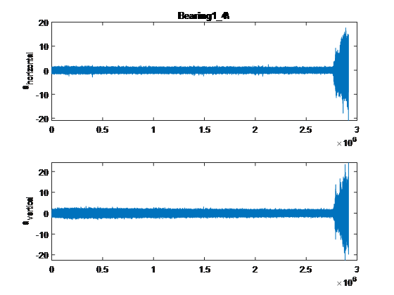
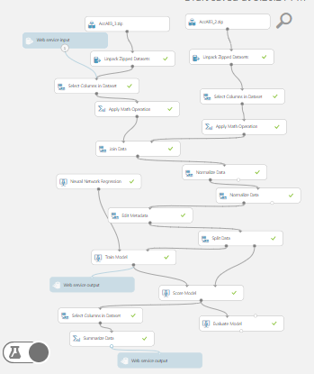
Table 1: Datasets for the IEEE 2012 PHM Prognostic Challenge

In Figure 7, the NNR model developed in the Microsoft Azure working studio is presented. The model, after running for a time limit of 20 seconds was set up to the web service that completed the task as shown in the figure, this was then used to predict the bearing dataset result.

The vibration signal obtained from the work was used for the prediction simulation. The summarized results of the Azure NNR model together with the Linear Regression Prediction for each bearing dataset folder are shown in Figures 8 – 11 and Table 2 respectively.

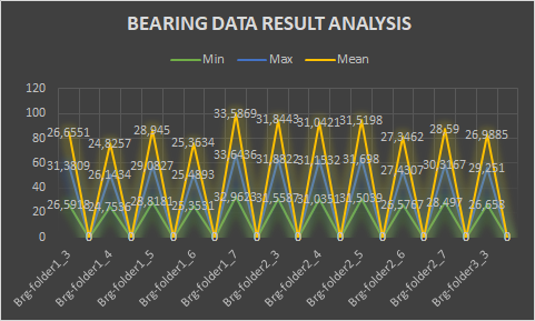
The highest mean was observed to be for the Bearing folder 1-7 folder dataset while the lowest mean value was found from the Bearing folder 1-4 dataset. The maximum value recorded was found to be for bearing folders 1-7 and the minimum value was recorded on Bearing folder 1-4. No outlier was observed or recorded.

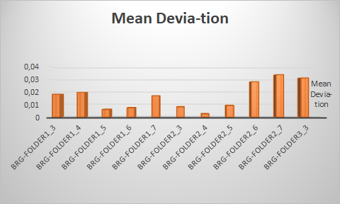
The lowest mean deviation was recorded for the Bearing folder 2-4 dataset, with the highest being recorded for the Bearing folder 2-7 dataset. Mean deviation is an important descriptive statistic which are not always found in quantitative statistics. This is primarily so because while mean deviation has a simple intuitive meaning as the “mean deviation from the mean”, the implementation of the absolute value makes empirical measurements far more complicated than the standard deviation using this statistic.

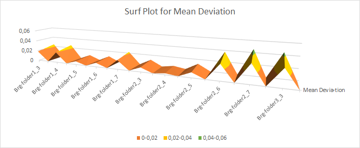
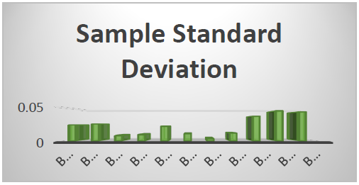
Figure 11 explicitly shows the sample standard deviation across the entire Bearing dataset.

In Table 2 is the actual experimental prediction result. The experiment percentage error is obtainable by the formula below:

$$\%Er_i = 100 \times \frac{ActRUL_i – \widehat{RUL}_i}{ActRUL_i} \tag{5}$$

Table 2: Actual Linear Regression Prediction

The actual datasets subject to experimentation or prediction are given in Table 2. The  for the datasets has been obtained from the simulation and the percentage error has been obtained and is shown in Table 3.

Table 3: The estimated

The RUL estimated score of accuracy for the experiments i is given as follows:

$$A_i = \begin{cases}
\exp^{- \ln(0.5) \cdot \left( \frac{Er_i}{5} \right)} & \text{if } Er_i \leq 0 \\
\exp^{+ \ln(0.5) \cdot \left( \frac{Er_i}{20} \right)} & \text{if } Er_i > 0
\end{cases} \tag{6}$$

The mean of all the experiment score defines the final score and this is given in the formula:

$$Score = \frac{1}{11} \sum_{i=1}^{11} A_i \tag{7}$$

5,537 sec was the predicted score from the use of both the NNR and Linear regression model.

6. Conclusion

Presented here in this paper is a suitable prediction method for big dataset-bearing behavior that needs no extra coding for the results attained from the test bed of the PRONOSTIA experiment. Also successfully done was the training of the model on the data obtained from the experiment, which helps to define the model’s strength. The Azure NNR model together with the use of statistical tools generated a reasonable judgmental result making this work accepted when compared to the other existing technique. Microsoft Azure Machine Learning work studio proves to be a fitting place to do condition monitoring forecasts without much coding expertise. This has made it a suitable means of evaluating the bearing frequency from their vibration signal.

It is also obvious that NNR when combined with known statistical tools forecasts better than linear regression models from the expected accuracy relative to previous results obtained. It is still possible to achieve better scores by using another model that requires more layers such as the deep neural network. Azure ML work studio has the capacity of working with data that are large as found applicable with other cloud computing platforms.

Conflict of Interest

The authors declare no conflict of interest.

Acknowledgment

I would like to acknowledge FEMTO- ST Institute (Franche-Comté ÉlectroniqueMécaniqueThermiqueetOptique – Sciences et Technologies) for the data sets they provided for this work and also for providing comprehensive reporting, including pictures of the bearing experiments to which the Result should be predicted.

1. H.O. Omoregbee; M.U. Olanipekun and B.A. Edward, “Non-Coding of Big Dataset and the use of Neural Network Regression Artificial Intelligence Model in Azure for Predicting the Remaining Useful Life (RUL) of Bearing,” IEEE AFRICON 2019, 1 – 7, 2019, doi: 10.1109/AFRICON46755.2019.9133738
2. G. Arminger and D. Enache “Statistical Models and Artificial Neural Networks,” In: Bock HH., Polasek W. (eds) Data Analysis and Information Systems. Studies in Classification, Data Analysis, and Knowledge Organization. Springer, Berlin, Heidelberg. 1996, https://doi.org/10.1007/978-3-642-80098-6_21
3. B. Li, M-Y., Chow, Y. Tipsuwan and J.C. Hung, “Neural-network-based motor rolling bearing fault diagnosis,” IEEE TRANSACTIONS ON INDUSTRIAL ELECTRONICS, 47(5), pp. 1060–1069. 2000, doi: 10.1109/41.873214
4. M. Chiarandini “Machine Learning : Linear Regression and Neural Networks,” in Introduction to Computer Science, Department of Mathematics & Computer Science, University of Southern Denmark.2017.
5. S. Bradley Russell, “A Comparison of Neural Network and Regression Models for Navy Retention Modeling,” Masters’ Thesis, Naval Postgraduate School, Monterey, CA 93943-5002.
6. A.K.B. Mahamad, “Diagnosis, Classification and Prognosis of Rotating Machine using Artificial Intelligence,” Kumamoto University Japan 2010.
7. R. G. Ahangar, “The Comparison of Methods Artificial Neural Network with Linear Regression Using Specific Variables for Prediction Stock Price in Tehran Stock Exchange,” International Journal of Computer Science and Information Security, 7(2), pp. 38–46, 2010, http://sites.google.com/sites/ijcsis/ ISSN: 1947 5500
8. K.A. Tsakiri and S. K. Marsellos, “Artificial Neural Network and Multiple Linear New York,” Molecular Diversity Preservation International, 10(1158), 2018, doi: 10.3390/w10091158.
9. O.S Maliki, A.O Agbo, A.O. Maliki, L.M Ibeh and C.O Agwu. “Comparison of Regression Model and Artificial Neural Network Model for the prediction of Electrical Power generated in Nigeria,” Pelagia Research Library, 2(5), pp. 329–339, 2011, www.pelagiaresearchlibrary.com ISSN: 0976-8610.
10. Z. Derouiche, M. Boukhobza, B. Belmekki and J.M. Rouvaen “Application of neural networks for monitoring mechanical defects of rotating machines,” in Proceedings of the 14th International Middle East Power Systems Conference (MEPCON’10), Cairo University, Egypt, December 19-21, 2010, Paper ID 161.
11. H.O. Omoregbee (2018), Diagnosis and prognosis of rolling element bearings at low speeds and varying load conditions using higher-order statistics and artificial intelligence, Ph.D. Thesis, Department of Mechanical and Aeronautical Engineering, University of Pretoria. South Africa.
12. D. An, J-H. Choi and N.H. Kim, “Remaining useful life prediction of rolling element bearings using degradation feature based on amplitude decrease at specific frequencies,” Structural Health Monitoring, 1–15, 2017, doi.org/10.1177/1475921717736226
13. W. Caesarendra, P.B. Kosasih, K. Tieu and Q. Zhu, “Acoustic emission-based condition monitoring methods: Review and application for low-speed slew bearing,” Mechanical Systems, and Signal Processing, 72-73, 2015, doi: 10.1016/j.ymssp.2015.10.020
14. K.A. Tsakiri and S. K. Marsellos, “Artificial Neural Network and Multiple Linear New York,” Molecular Diversity Preservation International, 10(1158), 2018, doi: 10.3390/w10091158.
15. C.L. Dunis, and J. Jalilov, (2002) “Neural Network Regression and Alternative Forecasting Techniques for Predicting Financial Variables by,” Neural network world, pp. 1–30. doi=10.1.1.335.7373&rep=rep1&type=pdf.
16. C-M. Lin, A-B.Ting, M-C.Li and T-Y. Chen, “Neural-network-based robust adaptive control for a class of non-linear systems,” Neural Comput&Applic, 20, pp. 557–563, 2011, doi: 10.1007/s00521-011-0561-2.
17. N. Zerhouni, C. Varnier, and P. An, “IEEE PHM 2012 Data challenge IEEE PHM 2012 Prognostic challenge Outline,” Experiment, Scoring of results, Winners (2012).

Citations by Dimensions

Citations by PlumX

Crossref Citations

1. Henry Ogbemudia Omoregbee, Mabel Usunobun Olanipekun, Bright Aghogho Edward, “Using Artificial Intelligence Models to Predict the Wind Power to be fed into the Grid”, Journal of Engineering Research and Sciences, vol. 3, no. 6, pp. 1–9, 2024. doi: 10.55708/js0306001
2. Henry Ogbemudia Omoregbee, Mabel Usunobun Olanipekun, Bright Aghogho Edward, “Evolutionary Learning of Fuzzy Rules and Application to Forecasting Environmental Impact on Plant Growth”, Journal of Engineering Research and Sciences, vol. 1, no. 4, pp. 48–53, 2022. doi: 10.55708/js0104006