Software-defined networking (SDN) represents an innovative approach to network architecture that enhances control, simplifies complexity, and improves operational efficiencies. This study evaluates the performance metrics of SDN frameworks using the Mininet simulator on virtual machines hosted on a Windows platform. The research objectives include assessing system performance across various predefined network topologies, investigating the impact of switch quantities on network performance, measuring CPU consumption, evaluating RAM demands under different network loads, and analyzing latency in packet transmission. Methods involved creating and testing different network topologies, including basic, hybrid, and custom, with the Mininet simulator. Performance metrics such as CPU and RAM usage, latency, and bandwidth were measured and analyzed. The study also examined the performance and extendibility of the OpenFlow Data Path (OFDP) protocol using the POX controller. Results indicate that balanced tree topologies consume the most CPU and RAM, while linear topologies are more efficient. Random topologies offer adaptability but face connection reliability issues. The POX controller and OFDP protocol effectively manage SDN network scalability. This research aims to analyze performance in a manner consistent with numerous previous studies, underscoring the importance of performance metrics and the scale of the network in determining the efficiency and reliability of SDN implementations. By benchmarking various topologies and protocols, the research offers a valuable reference for both academia and industry, promoting the development of more efficient SDN solutions. Understanding these performance metrics helps network administrators make informed decisions about implementing SDN frameworks to improve network performance and reliability.

1. Introduction

Networks are all around us, integral to our lives and daily routines. Most of the needs of a modern, technologically advanced society require strong and reliable networks. The demand for efficient networks is increasing exponentially with the passage of years and technological development. Nowadays, most people from all age groups use networks daily, and their quality of life depends on these networks, even if this is not immediately apparent. The COVID-19 pandemic that the world experienced from the beginning of 2020 changed many aspects of network usage. People were forced to spend much more time at home. This situation led people to find smart ways to meet most of their daily needs within the walls of their homes. Thus, the concept of the network in general came to everyone’s doorstep in the form of the largest known global network, the internet. Young people had to be educated remotely using the internet. Adults were mostly required to work from a distance, and the elderly and vulnerable groups had to seek their care and support in a different way with the help of the internet. This situation led to an unprecedented increase not only in the number of internet users but also in the number of different devices each user employs to access it. As a result, some weaknesses in the existing global networks were revealed, and new ones were created. Network providers and researchers realized that the capacity, speed, management, and reliability of networks needed to be increased due to the excessive load. Traditional networks that had been used for several years began to collapse because they primarily relied on physical infrastructures. Technologies such as SDN, which had been around for the last 10 years (mainly from 2013 onwards), began to be more extensively researched and implemented in global networks to strengthen them and ensure the smooth survival of the world. SDN enhances the capabilities of the network and simplifies its structure, with their main goal being more efficient network management. In this study, the architecture and structure of SDN networks will be examined. Network topologies will be created through simulations, and their operation and performance will be analyzed. Specifically, the performance between different topologies will be compared. It will be shown how the total number of switches, which are a fundamental pillar in the architecture of SDN, affects and burdens the overall performance of the network. The main measurements to be taken to draw accurate conclusions are CPU usage, RAM memory, and the delay in packet transfer between nodes. To achieve the above in the form of simulation, the Mininet simulator will be used on a computer with a Windows operating system. Additional software will be used in conjunction with Mininet to ensure the integrity and number of results. In this way, the behavior and adaptability of SDN networks will be studied. The controller used in Mininet will be POX, and further analysis will be done on the topology creation protocol OFDP, through which virtual networks will be studied below and their performance and scalability examined. The aim is to draw conclusions about the operation of SDN with the POX controller, specifically the use of the OFDP protocol. The reason for using random topologies is their effects on traditional networks and raises the question of how these random graphs can affect OpenFlow as its evolution into an even more modern network topology creation protocol. Given that network technologies have a strong relationship with network graphs and consequently with the concept of graph theory in mathematics, an analytical model for computation, comparison, and prediction is established through simulations on realistic platforms so that faster implementation in real-time networks can be achieved. The remainder of the article is as follows: Related search, SDN controllers, SDN protocols, Software & Hardware specifications, experiment specifications, analysis of results and finally the total conclusions from this research [1].

2. Related Search

Several research publications have been made on the aspect of SDNs, using the POX controller as well as OFDP for creating topologies. However, few utilize random topologies for interpreting SDN performance. In our previous research, we studied the performance results of Software-Defined Networking (SDN) tests conducted on standard network topologies using simulation. Concurrently, the performance of the standard topologies was compared with that of the random ones. Specifically, the performance measurements examined included: the setup and teardown time of the topology, the CPU and RAM usage of the system, and the delay in packet transfer between nodes. The entire study was conducted on a Windows computer using a virtual machine to run a Mininet simulator, similar to what we will use in the present work. From the meticulous analysis of the results, the following are worth mentioning: (i) the total number of switches in an SDN architecture has a significant impact on CPU load. (ii) RAM usage depends on the number of host computers and in cases of excessive load, it shows a much greater increase compared to CPU usage. (iii) The overall performance significantly depends on the type of topology and its properties. The experiments then were conducted on a typical and limited range of devices [2].

In his work, Guo created various types of network topologies for analysis, including ring topology, tree topology, and random Erdos-Renyi model topologies. In the randomly created networks, the probability of an edge between any two vertices was set at 0.4. Thus, these random networks were mostly dense networks with a short average path length. The ring networks had the longest average path length among the three topologies, while the tree topology was intermediate; all experiments were repeated 100 times. All nodes were subject to a common failure probability. Fifty nodes were used to create the three types of networks. The results show that the expected resilience of the network is inversely proportional to the average path length of the network topology, hence random topology networks perform better, and ring networks are less resilient [3].

In another study, the performance of the proposed discovery mechanism, which primarily relies on the OFDP protocol regarding the overall load, was analyzed. Various topologies were examined, focusing on random networks based on the Erdős–Rényi model. The study highlighted that researchers’ efforts are concentrated on reducing the number of messages reaching the controller. However, the performance and scalability of SDN networks depend more on other factors, such as CPU load, memory usage, network topology, and the time required for topology discovery. The scalability of OFDP and OFDPv2 for a wide range of random networks based on the Erdős–Rényi model was tested. Experimental results showed that the protocols consume almost equal resources (CPU and RAM), while OFDP requires more time for topology discovery than OFDPv2 for the same topology [4].

3. SDN Controllers

3.1. General SDN Information

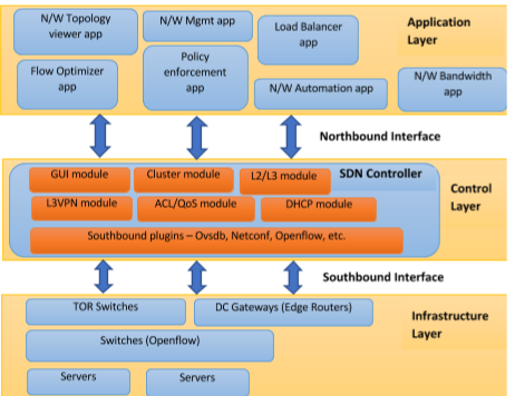
Software-Defined Networking (SDN) is a networking approach that uses software-based controllers or APIs to communicate with the underlying hardware infrastructure and direct traffic within a network. This model differs from traditional networks, which solely utilize hardware devices (routers and switches) to manage network traffic. SDN can create and manage a virtual network or control a traditional network through software. While network virtualization allows the segmentation of different virtual networks on a single physical network and the connection of devices across various physical networks to form a single virtual network, SDN enables a new method of controlling data packet routing through a central server. Consequently, SDN achieves the successful and functional separation of the Control Plane from the Forwarding Plane in a network. Below in Figure 1 the SDN architecture is depicted.

3.2. SDN Controller

A software-defined networking controller is a central element of the SDN architecture. It provides control over network elements in the managed domain. In networking, there are management, control, and data planes. An SDN controller offers management and control functions for network elements within the managed domain. This means that an SDN controller, based on network information and a set of predefined rules and policies, manages network elements and configures (or “programs”) the data plane (i.e., directs data flow through the network). One of the key advantages of using an SDN controller is that it allows for more efficient network management, and changes to the network configuration can be applied from a central location instead of needing to manually configure each individual network element. Additionally, an SDN controller can automate certain tasks, such as traffic management and security, which can reduce the risk of human error and improve the overall reliability of the network. SDN controllers provide an API known as the northbound interface, through which external applications or systems such as orchestration platforms can interact with the network. In such cases, an SDN controller translates application-level requirements (e.g., high-level network configuration description) into configurations specific to the supported network elements. SDN controllers can manage both physical network devices and software elements that perform network functions [6].

In summary, the main functions of an SDN controller include:

• Managing data flow within the managed network
• Providing an API for applications and other components (e.g., orchestration platforms) to interact with the network.
• Providing visibility into the network, enabling network performance monitoring and troubleshooting
• Automating network management tasks, such as provisioning new network elements and reconfiguring network paths

More specifically, the controller provides the following capabilities:

Southbound Support: Defined as how a controller interacts with network devices to achieve optimized traffic flow. There are various southbound protocols that can be used, each with specific functionalities such as field matching, network discovery with different protocols, etc. When supporting the southbound interface, implementers must consider not only the characteristics of the protocol but also potential extensions, newer versions, etc.

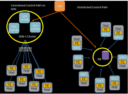
Northbound Support: Northbound APIs are used for network integration and programming and can be utilized by orchestration systems that cater to customers and third-party applications. It is crucial to ensure that a controller is properly developed for orchestrating communications between layers. For example, the controller should support orchestration systems for applications such as cloud services, not only for open-source controllers and protocols but also those provided by various vendors. These applications could also include traffic engineering or applications that collect data used for network management tasks. As we can see below in Figure 2 the differences between the structure of Centralized and Distributed control path are presented [7].

3.3.  NOX/POX Controller

NOX was the first SDN controller. Initially developed by Nicira Networks, it was the first to support the OpenFlow protocol. Released to the research community in 2009, it laid the foundation for many SDN research projects. It was later expanded and supported at Stanford University with significant contributions from the University of California, Berkeley. Some popular NOX applications include SANE (an approach that represents the network as a file system) and Ethane. Today, NOX is considered inactive. Over the years, different versions of NOX have been introduced. These are known as NOX, NOX-MT, and POX. The new NOX only supports C++. It has a smaller application network compared to NOX but is much faster and has a much cleaner codebase. NOX-MT, introduced as a slightly modified version of the NOX controller, uses optimization techniques to introduce multi-threaded processing to improve the rate and response time of NOX. These optimization techniques include I/O batching to minimize general input/output overhead and others. POX is the latest version based on Python. The idea behind its development was to return NOX to its roots in C++ and develop a separate platform based on Python. It also features a Python OpenFlow interface, reusable element samples for path selection, topology discovery, etc. The primary goal of POX is research. Given that many research projects are by nature short-lived, the focus of POX developers is on good interfaces rather than API stability. In the current research, due to the multiple interfaces and the stability of the controller and because the Python language was used to create network topologies, POX was used [8].

Generally, the NOX controller provides a complete OpenFlow API using C++ and Python languages, uses asynchronous inputs/outputs (I/O), and is oriented towards operation on Linux, Ubuntu, and Debian systems. NOX is used both as a standalone controller and as a component-based framework for developing SDN applications. It is built on an event-based programming model and adopts a simple programming interface model that revolves around three pillars:

• Events
• Namespace
• Network view

Events can be generated either directly from OpenFlow messages or from NOX applications because of processing low-level events or other events generated by applications.

4. SDN Protocols

The SDN protocol is a set of standards and rules that define how SDN controllers and switches communicate with each other. Essentially, a protocol allows the SDN controller to configure the behavior of the switch, such as determining which packets should be forwarded to which ports and setting quality of service (QoS) parameters for different types of traffic. The most popular SDN protocol is OpenFlow.

4.1. OpenFlow Protocol

As mentioned, OpenFlow is the most widespread SDN protocol and defines the flow between the switch and the controller. It allows the controller to manage traffic forwarding between different network devices by controlling the switch’s flow tables. This protocol was first developed by researchers at Stanford University in 2008 and was first adopted by Google in their backbone network in 2011-2012. It is now managed by the Open Networking Foundation (ONF). The latest version widely used in the industry is V1.5, while V2.0 is being refined. It is also often referred to as OFDP, meaning the OpenFlow Topology Discovery Protocol, because whether referred to as OpenFlow or OFDP, it automatically means the same function [9], [10].

OpenFlow is the standard southbound interface protocol used between the SDN controller and the switch. The SDN controller takes information from the applications and converts it into flow entries, which are fed into the switch via OpenFlow. It can also be used to monitor switch and port statistics in network management.

It is worth noting that the OpenFlow protocol is only installed between a controller and a switch. It does not affect the rest of the network. If a packet capture were to be taken between two switches in a network, both connected to the controller via another port, the packet capture would not reveal any OF messages between the switches. It is strictly for use between a switch and the controller. The rest of the network is not affected [11].

4.2. NetConf Protocol

NetConf is a protocol used in SDN for managing network devices such as routers and switches, providing a standardized way of configuring, monitoring, and managing these devices. It is an IETF standard and is based on XML data encoding and the SSH protocol for secure communication. The default TCP port assigned is 830. The NetConf server must listen for connections with the NetConf subsystem on this port.

With NetConf, network administrators can configure network devices programmatically using a standardized set of commands, rather than relying on proprietary interfaces for specific devices. This helps simplify network management and facilitates the automation of repetitive tasks such as deploying new network configurations or updates to hardware and software.

NetConf uses a client-server model, with the NetConf client sending requests to the device and the NetConf server responding with data or status updates. The protocol supports a range of functions, such as:

Retrieve: Retrieve specific data or configuration information from the device

Edit-config: Modify the device’s configuration.

Commit: Apply changes to the device’s configuration

Lock: Lock the device’s configuration to prevent multiple managers from making conflicting changes

Unlock: Release the configuration lock

NetConf is often used in conjunction with YANG, a data modeling language that allows network administrators to describe network elements and their configurations in a structured and standardized way. Together, NetConf and YANG form a significant component of SDN, enabling greater automation and control in network management.

4.3. Open vSwitch Database Management Protocol (OVSDB)

OVSDB is a protocol used in SDN networks for managing Open vSwitch instances, which are software-based switches that can be used in an SDN environment. OVSDB provides a standard way to configure and manage Open vSwitch instances, allowing network administrators to deploy and manage switches more automatically and programmatically. It defines a set of functions that can be used for querying and modifying the configuration of Open vSwitch instances, including creating, deleting, and modifying ports, interfaces, and VLANs.

OVSDB is based on a client-server model, with the OVSDB client sending requests to the OVSDB server, which responds with data or status updates. The protocol uses JSON data encoding and supports secure communication using TLS.

In an SDN environment, Open vSwitch instances can be used to forward traffic between different network devices and allow network administrators to manage traffic flows using a central SDN controller. OVSDB provides a standardized way to configure and manage these switches, facilitating the development and management of large-scale SDN networks.

4.4. Border Gateway Protocol (BGP)

BGP is a routing protocol commonly used in SDN networking environments to exchange routing information between different autonomous systems in large-scale networks. BGP is a path vector routing protocol that uses a network of interconnected autonomous systems to route traffic between different parts of the network.

In an SDN environment, BGP can be used to facilitate communication between different network elements, such as the SDN controller and network devices, or between different SDN controllers. BGP provides a standardized way to exchange routing information, allowing network managers to manage traffic flows and optimize network performance.

BGP uses a hierarchical routing table system, with each autonomous system maintaining its own routing table and exchanging updates with neighboring autonomous systems. The protocol supports both internal and external routing, allowing more efficient routing within a single autonomous system and between different autonomous systems [12].

4.5. Locator/Identifier Separation Protocol (LISP)

LISP is a protocol used in SDN to separate the network location of a device (essentially its IP address) from its identity or identifier. LISP provides a way to assign multiple IP addresses to a device and allows routing of traffic based on the device’s identity rather than its physical location.

In an SDN environment, LISP can be used to simplify network management and enable more efficient routing of traffic between different devices. By separating the device’s identity from its location, LISP allows network administrators to move devices between different network locations without changing their IP addresses, simplifying network management and reducing the likelihood of errors [13].

4.6. Simple Network Management Protocol (SNMP)

SNMP is a protocol used in software-defined networking (SDN) for monitoring and managing network devices. SNMP provides a standardized way for network administrators to monitor the performance of network devices, such as switches and routers, and to configure them remotely.

In an SDN environment, SNMP can be used to monitor and manage network devices from a central SDN controller. SNMP allows network administrators to monitor a range of device metrics, such as CPU usage, memory usage, and network traffic, and to receive alerts when performance issues arise.

SNMP is based on a client-server model, with SNMP agents running on network devices and SNMP managers running on the SDN controller. The agents collect performance data and send it to the managers, who can then analyze the data and take actions to improve network performance.

SNMP is a widely used protocol in network management and is supported by a range of network device suppliers and SDN controllers. It can be used in conjunction with all the above-mentioned SDN protocols to enable more effective and flexible network management.

4.7. Link Layer Discovery Protocol (LLDP)

LLDP is a Layer 2, vendor-neutral protocol used for discovering and advertising network device information on a local area network (LAN). It allows network devices to exchange information about their identity, capabilities, and connections [14].

LLDP operates by sending and receiving LLDP frames, which are multicast packets transmitted on every network interface. LLDP frames contain TLV (Type-Length-Value) elements that carry specific information about the transmitting device, such as system name, port description, system capabilities, and management addresses.

Key features and benefits of LLDP include:

Device Discovery: LLDP enables network devices to discover neighboring devices on the LAN, providing information about their identity, such as device type, vendor, and model.

Topology Discovery: By exchanging LLDP information, devices can gather details about the connections and topology of the network, including neighboring devices, port numbers, and connection speeds.

Automatic Configuration: LLDP can be used by network management systems to automatically configure network devices based on their discovered capabilities, simplifying network setup and reducing the efforts of manual configuration.

Troubleshooting and Monitoring: LLDP facilitates network troubleshooting by providing visibility into the network topology and device connectivity. It allows administrators to identify and locate devices, detect link failures, and monitor the status of connections.

LLDP is supported by a wide range of network devices, including switches, routers, wireless access points, and IP phones. It is often used in conjunction with other network protocols, such as SNMP, to enable comprehensive network management and monitoring.

It is important to note that LLDP is a Layer 2 protocol, and its functionality is limited to the local network segment. It does not route traffic nor provide visibility into the entire network.

4.8. Advantages of SDN

Software-defined networking (SDN) has emerged as a transformative approach to network architecture and management. By decoupling the control plane from the data plane and centralizing network control through software, SDN provides numerous benefits and impacts various industries. Key findings on SDN include:

• Enhanced Network Flexibility: SDN allows organizations to quickly provision, configure, and modify network services via software, leading to improved network flexibility. It enables dynamic allocation of network resources, making it easier to adapt to changing business needs and network traffic patterns [15].
• Simplified Network Management: SDN centralizes network management through a software-managed controller, providing a single point of control and monitoring. This simplifies network management, reduces complexity, and enhances troubleshooting capabilities.
• Scalability and Flexibility: SDN offers scalability by abstracting network functionality from the underlying hardware. Organizations can more easily scale their networks by adding or reallocating resources according to needs. Furthermore, SDN allows flexibility in deploying new services and applications without significant changes to infrastructure.
• Network Programmability: SDN enables network programmability, allowing administrators to automate network functions and control network behavior through software. This programmability facilitates the development of innovative applications and services that can interact directly with the network.
• Enhanced Security: SDN provides enhanced security capabilities by leveraging centralized control and programmability. Security policies can be defined and enforced consistently across the network, making it easier to identify and respond to threats.
• Cost Optimization: SDN offers cost savings by reducing hardware dependencies and enhancing resource utilization. With the ability to dynamically control and distribute network resources, organizations can optimize their infrastructure, leading to better cost performance.
• Innovation and Ecosystem Development: SDN promotes innovation by enabling the development of new network services and applications. It encourages the development of an ‘ecosystem’ where vendors, developers, and researchers can collaborate to create new solutions and advance networking progress.
• SD-WAN and Cloud Connectivity: SDN plays a critical role in the adoption of software-defined wide area networks (SD-WAN) and in connecting on-premises networks to cloud environments. It simplifies the management of distributed networks, provides better visibility and control, and improves connectivity to cloud services.

4.8. challenges and issues

While SDN offers significant benefits, it also presents challenges, including interoperability among different SDN solutions, security concerns related to centralized control, the need for specialized personnel to manage and operate SDN environments, and the necessity for careful planning, testing, and collaboration with experienced vendors to overcome these challenges.

SDN Protocols:

• SDN protocols play a critical role in the implementation and operation of software-defined networking (SDN) environments. These protocols define the communication and interaction between different elements of an SDN architecture, facilitating network control and management.
• OpenFlow is one of the most widely adopted SDN protocols. It provides a standard interface between the control layer and forwarding devices (switches). OpenFlow enables centralized network control by separating control logic from switches and allowing the controller to program forwarding rules. It has significantly contributed to the development and deployment of SDN solutions.

SDN Controllers:

• SDN controllers serve as the central intelligence of software-defined network (SDN) architectures. They are responsible for managing and orchestrating network resources, facilitating communication between the control layer and the data layer, and enabling network programmability.

Table 1: below presents the network protocols along with their pros and cons.

Table 1: Network protocols.

5. Software & Hardware specifications

In this section, we will analyze each tool used for this work. Specifically, both the hardware and software components will be discussed.

5.1. Hardware Specifications

Compared to previous related research where high-performance laptops, low-performance desktops, or even workstations were used, this research utilized a new high-performance desktop computer. This system offers the capability to implement larger virtual networks as well as optimized management and distribution of physical resources, allowing for improved performance and more efficient scaling of the networks that will be created. In the heart of the computing system used for this research, the Gigabyte B550M AORUS PRO motherboard with an AMD B550 chipset lays the foundation. This motherboard was chosen for its robust support for modern connectivity standards such as PCI EXPRESS 4.0, which is pivotal for high-performance setups required in advanced simulations and experiments. The AMD Ryzen 5 5600X processor, featuring a 7nm FinFET technology with 6 cores and 12 threads, is selected for its ability to handle extensive computations more effectively than comparable models used in preceding studies. Its overclocking ability up to 4.7 GHz facilitates faster processing of complex tasks, crucial for developing larger virtual networks and conducting intensive data analysis.

Additionally, the system is equipped with 32GB of DDR4 RAM at 3600 MHz in dual-channel configuration, providing ample bandwidth and speed necessary for managing multiple operations simultaneously, which is essential when testing the limits of network simulations and other resource-intensive applications. The AMD Radeon RX 6750 XT graphics card with 12GB of GDDR6 memory ensures smooth rendering of complex graphics and supports the visualization demands of the research, including the manipulation and analysis of high-dimensional data sets.

Storage is handled by a Kingston KC3000 NVMe SSD with a capacity of 2TB, leveraging PCI Express 4.0 technology to offer rapid data access speeds of up to 7000 MB/s, significantly reducing load times and improving the overall efficiency of data processing tasks. This storage solution is vital for handling large volumes of data generated during simulations, ensuring quick retrieval and processing that are imperative for maintaining workflow continuity during the research.

Together, these hardware specifications are meticulously chosen not only for their individual capabilities but also for their synergy, which ensures a high-performance, stable, and reliable computing environment capable of supporting the sophisticated software tools and simulations utilized in this research. In Table: 2 we have the technical specifications of our systems.

Table 2: Simulation system specifications.

5.2. Software Specifications

In this section, the specifications of the system software used are analyzed. It is crucial not only to conduct research to use the correct software that can deliver the desired results but also to ensure that all software can work harmoniously together. Cohesion, relevance, and repeated checks on the outcomes that will be extracted are necessary. For the software setup in this research, specific tools have been meticulously selected to complement the powerful hardware configuration and to meet the specialized requirements of the study. The primary operating system used is Windows 11 Pro for Workstations, which offers essential features like the ReFS file system for enhanced data resilience and support for advanced hardware configurations, critical for maximizing the potential of the system’s physical components.

Oracle’s VirtualBox plays a key role by allowing the deployment of multiple operating systems on a single physical machine, which is crucial for testing different network configurations and software interactions in a controlled, isolated environment. This flexibility is vital for reproducing and manipulating network scenarios in the development of software-defined networking (SDN) solutions.

Additionally, Visual Studio Code is employed as the primary code editor due to its robust support for multiple programming languages and its integrated development environment (IDE) features like debugging, code completion, and Git integration. These features enhance the efficiency of writing and testing code, particularly Python scripts used for creating network topologies in the research.

Gephi, an open-source network visualization software, is used to analyze and visualize complex network structures, which helps in understanding the interactions within the network and identifying key patterns and anomalies. The ability to dynamically model network traffic and topology changes in real-time using Gephi significantly aids in the exploratory phase of the research.

Furthermore, the inclusion of specialized tools like PuTTY for secure remote session management, WinSCP for secure file transfer, and Xming for running X Window System applications on Windows, consolidates the software environment.

Together, these software tools form a cohesive ecosystem that supports the rigorous demands of the research, enabling sophisticated simulations, extensive data analysis, and effective management of resources across different stages of the project. Table 3 contains an analysis of all the software used.

Table 3: Simulation software presentation.

6. Experiment Specifications

6.1. Network Topologies

The term topology defines the geometric representation of the connections in a network. We examined three categories of topologies.

• Basic
• Hybrid
• Custom

Specifically, for the basic topologies, the bus topology was selected, for the hybrid topologies, the balanced tree topology was chosen, and for the Custom, the random topology was used [16], [17].

6.1.1. Basic Topologies

There are many basic network topologies commonly used in computer networking. These include:

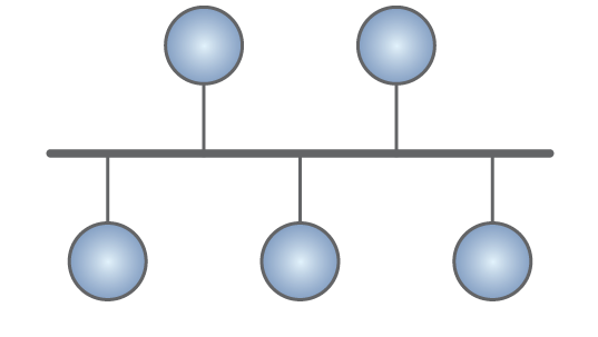
Bus topology: All devices are connected to a single communication line or cable, known as the bus. Data travels in both directions along the bus and all devices on the network can receive the same message simultaneously. Figure 3 depicts bus topology.

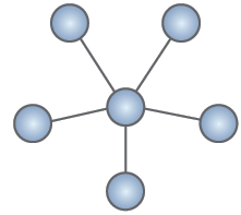
Star topology: All devices are connected to a central hub or switch, and data flows through the hub or switch to reach its destination. Each device has an exclusive connection to the hub or switch, which can help reduce network congestion and improve performance. Figure 4 depicts star topology.

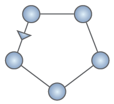
Ring topology: All devices are connected in a closed loop, with data flowing in one direction around the loop. Each device receives data from the previous device in the loop and sends data to the next device in the loop. The ring topology is depicted in Figure 5 below.

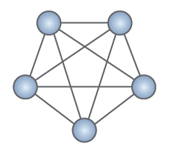
Mesh topology: Each device is connected to every other device in the network, creating a fully interconnected network. This can provide high redundancy and fault tolerance but can be complex to manage and requires a lot of wiring. Figure 6 presents mesh topology.

6.1.2. Hybrid Topologies

Hybrid Topology is a combination of two or more basic topologies, such as a star-bus topology or a ring-mesh topology. This can offer a balance between performance, redundancy, and ease of management.

Tree topology, also known as hierarchical topology, is a type of network topology based on a hierarchical structure. In this topology, multiple star topologies relate to a bus topology, creating a structure that resembles a tree. In a tree topology, the central bus acts as the main trunk of the tree, with multiple branches extending from it. Each branch is a separate star topology with a hub or switch at the center and multiple devices connected to it. This allows the creation of subnetworks within the larger network, with each subnet having its own exclusive hub or switch.

The main advantage of a tree topology is its scalability, as it can support many devices and subnetworks. It also provides a good balance between performance and redundancy, as each subnet can operate independently and problems in one subnet will not affect the rest of the network.

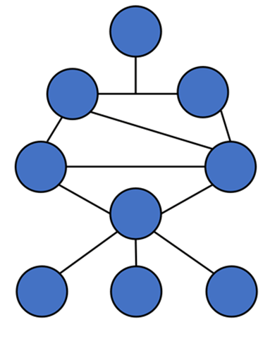
However, the main disadvantage of a tree topology is its complexity, as it requires a significant amount of cabling and configuration. It can also be difficult to troubleshoot and manage, as problems in one part of the network can affect the entire tree. Below in Figure 7 an example of hybrid topology can be found.

A balanced tree topology is a specific type of tree topology where each branch of the tree has the same number of levels. This means that each subnet is of equal size and has the same number of devices connected to it. In a balanced tree topology, the central bus is connected to a set of level-1 switches, each of which is connected to a set of level-2 switches, and so on, until the final level of switches is reached. Each switch in the tree has an equal number of branches connected to it, which helps balance the network traffic and avoid congestion.

6.1.3. Custom Topologies

Custom network topologies refer to network architectures designed to meet specific requirements or solve specific problems. They may be a combination of two or more basic topologies, or they may be entirely unique and tailored to a specific application or environment. Custom network topologies can be created by network designers and administrators using various networking devices and technologies, such as switches, routers, firewalls, load balancers, and others. These devices can be configured to implement specific routing protocols, VLANs, access control policies, and other features to achieve the desired network behavior and performance. Examples of custom network topologies include:

Mesh topology with adaptive routing: This topology can be used in large-scale wireless networks to provide high redundancy and fault tolerance. Adaptive routing protocols such as OLSR or B.A.T.M.A.N. may be used to optimize network performance and reduce congestion. Hub-and-Spoke topology with VPN: This topology can be used to connect multiple remote offices or branches to a central location using VPN tunnels. A hub router or firewall is used to manage the traffic flow and provide secure connectivity between the spokes.

Cluster topology with load balancing: This topology can be used to create a cluster of web or application servers for high availability. Load balancing devices are used to distribute traffic across multiple servers in the cluster, providing high performance and scalability.

Custom network topologies can offer unique advantages and solve specific problems, but they also require careful design and management to ensure effectiveness and security. Network administrators should consider the specific needs of their organization and consult experienced network designers to create a custom topology that meets these needs.

6.1.4. Random Topology

In computer networking, a random network topology refers to a network topology where connections between nodes are made in a random or stochastic manner. In such a topology, there is no predetermined plan or structure to the connections between nodes. Random network topologies are used in various applications, such as in the study of social networks, biological networks, and communication networks. They are also used in analyzing network properties, such as connectivity, robustness, and efficiency. It has been shown that they exhibit some interesting and unexpected behaviors, such as the emergence of small-world networks and scale-free networks.

6.1.5. Erdős–Rényi Model

An example of a random network topology is the Erdős–Rényi model. The Erdős–Rényi model, also known as the ER model, is a mathematical model for creating random graphs. Introduced to the field of mathematics by mathematicians Paul Erdős and Alfréd Rényi in 1959, the ER model creates a random graph with “n” nodes starting with “n” isolated nodes and then randomly connecting pairs of nodes with a certain probability “p”. The edges between the nodes are independent and occur with probability “p”. There are two variations of the ER model: the G(n,m) model, which creates a random graph with “n” nodes and m edges, and the G(n,p) model, which creates a random graph with “n” nodes and an edge between each pair of nodes with probability “p”.

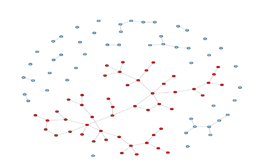
The ER model has been used to study various properties of random graphs, including the appearance of the giant component, the phase transition of connectivity, and the degree distribution of the graph. The model has also been applied in various fields such as social networks, computer networks, and biology. However, it should be noted that the ER model assumes a completely random and uniform distribution of edges, which may not always reflect the real structure of many networks. As a result, other network models, such as small-world networks and scale-free networks, have been proposed to better map the properties of real networks. In Figure 8 below we can see a custom random topology is presented [18].

6.2. Experiment Specifications

The experiments implement topologies based on the random topology which in turn follows the Erdős–Rényi mathematical model. The SDN controller used is POX due to its compatibility with both topologies and the creation and parameterization of topologies through the PYTHON language. The topology creation protocol is OFDP, or otherwise OpenFlow [19].

The experiments examine the following:

• Comparison of system performance according to topologies.
• Comparison of system performance according to topology creation protocol.
• Comparison of system performance according to the number of switches and how the total number of switches affects performance.
• CPU usage.
• RAM usage
• The delay of packet transfer between network nodes.
• The time of creation and destruction of a topology

The above measurements will be compared:

Topologies:

• Linear
• Balanced Tree
• Random Topology

Creation Protocols

• OFDP
• LLDP
• BGP
• LSDP
• SNMP
• OVSDB

The number of switches will remain steadily increasing, and each switch will be connected to a host in the manner shown in the table below [20].

It is noted that a greater number of switches was achieved than in most similar studies. This fact alone allows for better interpretation of results and is primarily due to the available hardware resources. Table 4 contains the scale of the experiments depending on the number of switches and hosts.

Table 4: Scale of experiments conducted

6.3. Collection of General Results

In this section, the statistical tables of the data collected from the above experiments will be presented. The controller used is POX and the topology creation protocol is OFDP. It is worth noting that each experiment was performed about a thousand times to ascertain the accuracy percentage of the results, and the deviations were minimal and consistent with the expected pattern. Therefore, the results presented are the overall average. Below the tables of experiment results are presented. Table 5 presents the results using random topologies, Table 6 presents the results using linear topologies and Table 7 presents the results using balanced tree topologies [21].

Table 5: Experiment results using random topologies.

Table 6: Experiment results using linear topologies.

Table 7: Experiment results using balanced tree topologies.

6.3.1. Collection of Latency Results

Latency measurement will be done differently as each network is measured under similar conditions with a fixed packet size, increasing the number of packets and observing how this affects the network. The average and total transfer times are collected. The size of each packet is defined as 1024Bytes (1KB), and simulations will be executed with the corresponding packet numbers [1,10,50,100,500]. In previous studies, a usage limit of about 600 packets of this packet size was observed in Mininet. Below Table 8 is presented in which we can see the latency results of each topology.

Table 8: Latency results of experiments across all topologies.

7. Analysis of results

The results obtained in the present research are appropriately transformed into diagrams. On the vertical axis, each studied element (CPU, RAM, Bandwidth, Setup Time, Tear Time, Latency) is distributed, while on the horizontal axis there is the number of switches used, thus conclusions are drawn based on the quantity of Switches. In the Latency diagram, on the horizontal axis, the number of Switches is replaced by the number of packets.

7.1. CPU Analysis

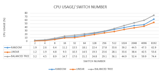
The following section provides an in-depth analysis of CPU usage in relation to the number of switches in various network topologies. The data illustrates that CPU usage increases as the number of switches rises. The analysis is based on comparative data from three topologies: balanced tree, random, and linear.

7.1.1. Balanced Tree Topology

Highest CPU Consumption: The balanced tree topology consumes the most CPU resources among the three topologies. This is attributed to the complexity and structure of the tree-branches, which require more processing power to manage the available paths.

CPU Usage Increases with Switches: As the number of switches increases, CPU usage significantly rises. At the peak of 8192 switches, the CPU usage reaches 74.4%, which is 11.5% higher than the random topology and 20.8% higher than the linear topology.

7.1.2. Random Topology:

Close to Balanced Tree: The random topology’s CPU consumption is slightly less than the balanced tree but higher than the linear topology. This is due to the adaptable nature of the random topology, which requires complex computations to manage dynamic connections.

Instabilities: Some instabilities in CPU usage are observed, caused by the probability of unsuccessful connections between nodes, which adds variability to the CPU load.

7.1.3. Linear Topology

Least CPU Usage: The linear topology demonstrates the least CPU usage due to its simple and straightforward connectivity. The simplicity of managing linear connections results in lower processing requirements.

Stable Performance: The linear topology shows stable CPU performance, with less variability and lower overall CPU consumption compared to the other topologies.

Complexity and Resource Allocation: The balanced tree topology requires more CPU resources due to its hierarchical structure. Managing multiple levels and branches in the network involves more processing to maintain efficient routing and data flow. This complexity inherently increases the CPU load as the network scales.

Adaptability of Random Topology: While the random topology is designed for flexibility and adaptability, this also introduces challenges in maintaining stable connections. The CPU must handle dynamic routing and potential connection failures, leading to increased CPU usage and occasional spikes.

Efficiency of Linear Topology: The linear topology benefits from its simplicity, where each switch is directly connected in a straightforward path. This minimizes the processing required for routing decisions, leading to lower and more consistent CPU usage. The linear approach simplifies network management and reduces the computational burden on the CPU.

The analysis highlights that network topology significantly impacts CPU usage. The balanced tree topology, while offering robust and hierarchical structuring, imposes a high CPU load due to its complexity. The random topology, though adaptable, faces challenges with connection stability, leading to variable CPU consumption. Linear topology remains the most efficient in terms of CPU usage, owing to its simple and direct connectivity. These findings are crucial for network administrators and designers, emphasizing the need to consider topology choice based on the expected network load and performance requirements. Balancing complexity, adaptability, and efficiency is key to optimizing network performance and resource utilization. Figure 9 analyses the CPU usage in each experiment.

7.2. RAM Analysis

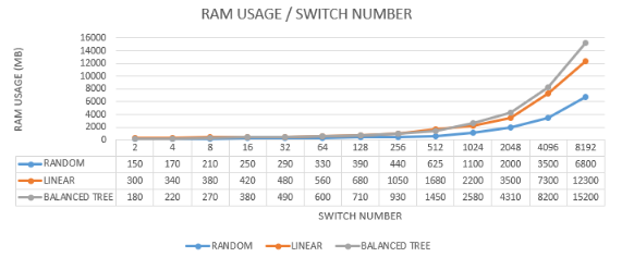
The following section provides an in-depth analysis of RAM usage in relation to the number of switches in various network topologies. The data illustrates that RAM usage varies significantly with the topology used and the number of switches in the network. This analysis is based on comparative data from three topologies: linear, balanced tree, and random.

7.2.1. Linear Topology

Initial High Memory Consumption: Initially, the linear topology consumes more RAM compared to the other two topologies, despite using less CPU than the balanced tree. This higher initial memory usage can be attributed to the straightforward but memory-intensive nature of maintaining direct connections between each switch.

Memory Usage Trends: As the number of switches increases, the memory usage grows but at a predictable and steady rate due to the simple structure of the linear topology.

7.2.2. Balanced Tree Topology

High Memory Consumption with Increased Switches: While the number of switches increases, the balanced tree topology eventually consumes the most memory. This is due to the complexity of managing a hierarchical tree structure, which requires more memory to store the state and routing information for multiple levels and branches.

Complexity Impact: The tree-branch structure inherently requires more memory to maintain the hierarchical relationships and efficient routing, resulting in higher memory usage as the network scales.

7.2.3. Random Topology

Lowest Memory Consumption: The random topology consistently shows lower RAM usage compared to the other two topologies. This is largely due to its customization and the retrospective improvements made to its implementation in Mininet, which optimize memory usage.

Efficiency of Customization: Due to its adaptable nature and optimized design, the random topology reduces memory consumption by about 45-55% compared to the linear and balanced tree topologies.

Initial Memory Usage in Linear Topology: The linear topology, despite its simplicity, requires substantial memory initially to establish and maintain direct connections between each switch. This direct approach, while less CPU-intensive, places a higher initial burden on RAM.

Increasing Complexity in Balanced Tree Topology: As the network grows, the balanced tree topology’s memory requirements increase significantly. This is because the hierarchical structure demands more memory to store the details of each level and branch, ensuring efficient data routing and network management.

Optimized Memory Usage in Random Topology: The random topology benefits from its customized and optimized implementation in Mininet. This design reduces unnecessary memory usage and streamlines the management of random connections, leading to significantly lower RAM consumption. The flexibility and adaptability of the random topology also contribute to its efficient memory usage.

The analysis highlights that network topology significantly impacts RAM usage. The linear topology, while simple, initially demands more memory but grows predictably. The balanced tree topology, due to its hierarchical structure, consumes the most memory as the network expands. The random topology, with its optimized and adaptable design, demonstrates the most efficient memory usage. These insights are crucial for network administrators and designers, emphasizing the need to consider topology choice based on the expected network load and performance requirements. Balancing complexity, adaptability, and efficiency is key to optimizing network performance and resource utilization, particularly in terms of memory usage. Figure 10 analyses the RAM usage in each experiment.

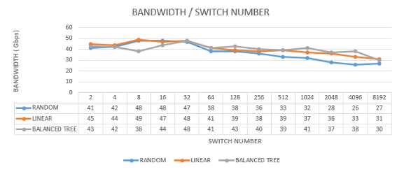
7.3. Bandwidth Analysis

The following section provides an in-depth analysis of RAM usage in relation to the number of switches in various network topologies. The data illustrates that RAM usage varies significantly with the topology used and the number of switches in the network. This analysis is based on the comparative data from three topologies: linear, balanced tree, and random.

7.3.1. Linear Topology

Initial High Memory Consumption: Initially, the linear topology consumes more RAM compared to the other two topologies, despite using less CPU than the balanced tree. This higher initial memory usage can be attributed to the straightforward but memory-intensive nature of maintaining direct connections between each switch.

Memory Usage Trends: As the number of switches increases, the memory usage grows but at a predictable and steady rate due to the simple structure of the linear topology.

7.3.2. Balanced Tree Topology

High Memory Consumption with Increased Switches: While the number of switches increases, the balanced tree topology eventually consumes the most memory. This is due to the complexity of managing a hierarchical tree structure, which requires more memory to store the state and routing information for multiple levels and branches.

Complexity Impact: The tree-branch structure inherently requires more memory to maintain the hierarchical relationships and efficient routing, resulting in higher memory usage as the network scales.

7.3.3. Random Topology

Lowest Memory Consumption: The random topology consistently shows lower RAM usage compared to the other two topologies. This is largely due to its customization and the retrospective improvements made to its implementation in Mininet, which optimize memory usage.

Efficiency of Customization: Due to its adaptable nature and optimized design, the random topology reduces memory consumption by about 45-55% compared to the linear and balanced tree topologies.

Initial Memory Usage in Linear Topology: The linear topology, despite its simplicity, requires substantial memory initially to establish and maintain direct connections between each switch. This direct approach, while less CPU-intensive, places a higher initial burden on RAM.

Increasing Complexity in Balanced Tree Topology: As the network grows, the balanced tree topology’s memory requirements increase significantly. This is because the hierarchical structure demands more memory to store the details of each level and branch, ensuring efficient data routing and network management.

Optimized Memory Usage in Random Topology: The random topology benefits from its customized and optimized implementation in Mininet. This design reduces unnecessary memory usage and streamlines the management of random connections, leading to significantly lower RAM consumption. The flexibility and adaptability of the random topology also contribute to its efficient memory usage.

The analysis highlights that network topology significantly impacts RAM usage. The linear topology, while simple, initially demands more memory but grows predictably. The balanced tree topology, due to its hierarchical structure, consumes the most memory as the network expands. The random topology, with its optimized and adaptable design, demonstrates the most efficient memory usage. These insights are crucial for network administrators and designers, emphasizing the need to consider topology choice based on the expected network load and performance requirements. Balancing complexity, adaptability, and efficiency is key to optimizing network performance and resource utilization, particularly in terms of memory usage. Figure 11 analyses the bandwidth of each experiment.

7.4. Setup Time Analysis

The setup time refers to the duration required to create a network topology, measured from the moment the creation command is initiated. The analysis compares the setup times for three different network topologies: random, balanced tree, and linear. The results indicate significant differences in the time taken to establish each topology, highlighting the efficiency and complexity involved in their creation.

7.4.1. Random Topology

Longest Setup Time: The random topology consistently shows the longest time required to create a topology. This is due to its inherent complexity and the need for random connections between nodes, which involves additional computational overhead to ensure successful creation and connectivity.

Marginally Longer: Among the topologies with long setup times, the random topology takes slightly longer than the balanced tree, indicating higher variability and complexity in establishing random connections.

7.4.2. Balanced Tree Topology

Long Setup Time: The balanced tree topology also exhibits a long setup time, slightly less than the random topology. The hierarchical structure requires careful planning and execution to ensure all branches and levels are correctly established, which adds to the setup time.

Complexity Contribution: The structured nature of the balanced tree, with multiple levels and branches, contributes to the extended time needed for its creation.

7.4.3. Linear Topology

Shortest Setup Time: The linear topology shows a significantly reduced setup time compared to the other two topologies. This is due to its straightforward design, where each node is directly connected to the next in a simple chain.

Efficiency in Large Networks: In very large networks, the linear topology is approximately 30-40% faster to set up than the random and balanced tree topologies. This efficiency is attributed to the minimal complexity in establishing direct connections sequentially.

Complexity and Overhead: The random and balanced tree topologies require more time to create due to their inherent complexity. Random topology involves the creation of non-deterministic connections that need verification and correction, while the balanced tree requires a hierarchical setup with multiple levels, each adding to the overall setup time.

Linear Topology Efficiency: Linear topology’s setup process is inherently simpler. Each new node is added in a straightforward manner, reducing the time required for planning and establishing connections. This simplicity translates to a significant reduction in setup time, especially as the network scales.

Scalability and Performance: As the network size increases, the difference in setup times becomes more pronounced. The linear topology’s efficient setup process becomes increasingly advantageous in larger networks, where the time savings are substantial compared to the more complex topologies.

Practical Implications: For practical applications, the choice of topology can significantly impact the time required to deploy a network. In scenarios where rapid deployment is critical, the linear topology offers a clear advantage. Conversely, if the network’s structural complexity and adaptability are priorities, the additional setup time for random or balanced tree topologies may be justified.

The setup time analysis underscores the importance of topology selection based on deployment time requirements and network complexity. The linear topology offers the fastest setup time, making it suitable for scenarios requiring quick deployment and straightforward management. The random and balanced tree topologies, while taking longer to set up, provide more complex and potentially more resilient network structures. Understanding these trade-offs is essential for network administrators and designers to optimize network deployment strategies and achieve the desired balance between setup efficiency and structural complexity. Figure 12 show the results of setup time of the experiments.

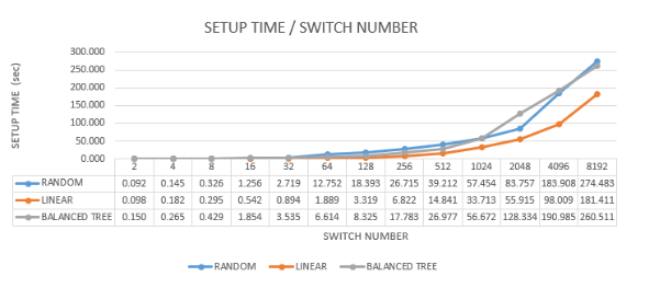
Figure 12: Comparative setup time diagram for the three topologies

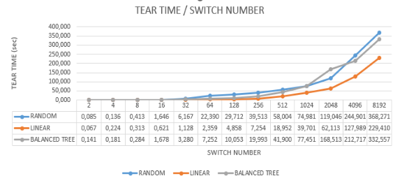
7.5. Tear Time Analysis

The tear time refers to the duration required to dismantle a network topology, measured from the moment the destruction command is initiated. The analysis compares the tear times for three different network topologies: linear, balanced tree, and random. The results indicate significant differences in the time taken to dismantle each topology, highlighting the efficiency and complexity involved in their destruction.

7.5.1. Linear Topology

Shortest Tear Time: As expected, the linear topology takes the least amount of time to tear down. This is due to its straightforward structure, where nodes are connected in a simple chain, making it easy to dismantle.

Efficiency in Large Networks: In large networks, the linear topology shows about 30-40% faster tear times compared to the random and balanced tree topologies. This efficiency is attributed to the minimal complexity involved in breaking the direct sequential connections.

7.5.2. Random Topology

Longest Tear Time: The random topology consistently shows the longest tear time among the three topologies. This is due to the complexity and unpredictability of its connections, which require additional time to ensure all links are properly dismantled.

Peak Tear Times: The tear time peaks higher in the random topology, reflecting the inherent variability and instability in its structure.

7.5.3. Balanced Tree Topology

Long Tear Time: The balanced tree topology also exhibits a long tear time, like the random topology but slightly less. The hierarchical structure requires careful dismantling of multiple levels and branches, adding to the overall tear time.

Deviations in Linearity: Some deviations in the linearity of tear time are observed in the balanced tree topology. These deviations are due to the changes in the tree structure as different branches and levels are dismantled.

Efficiency of Linear Topology: The linear topology’s simplicity extends to its tear-down process. Each node is directly connected to its predecessor and successor, making it easy to break these connections in sequence. This straightforward dismantling process results in consistently lower tear times.

Complexity in Random Topology: The random topology’s longer tear time is attributed to its complex and unpredictable nature. The random connections between nodes mean that each dismantling process is unique and requires more time to ensure all links are effectively broken. This variability results in higher and more inconsistent tear times.

Structured Dismantling in Balanced Tree Topology: The balanced tree topology requires careful dismantling of its hierarchical structure. Each branch and level must be carefully broken down, which increases the overall tear time. The deviations in linearity are due to the varying complexity of dismantling different parts of the tree.

Instabilities and Variability: Both the random and balanced tree topologies show instabilities and variability in tear times. These instabilities are natural given the complexity of the structures and the need for careful dismantling to avoid leaving residual connections.

The tear time analysis highlights the impact of network topology on the efficiency of dismantling processes. Linear topology offers the fastest and most efficient tear-down times, making it suitable for scenarios requiring quick and straightforward network reconfiguration. The random and balanced tree topologies, while offering more complex and potentially more resilient structures, require significantly more time to dismantle. Understanding these differences is crucial for network administrators and designers in optimizing network management strategies, particularly in environments where frequent reconfiguration is necessary. Figure 13 show the results of tear time for each experiment.

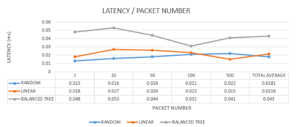
7.6. Latency Analysis

Latency measurement refers to the time taken for an information packet to travel from one network node to another, measured in milliseconds (ms). For this analysis, the packet size was set to 1024 Bytes (1 Kilobyte), and the maximum number of transferred packets was capped at 500, a limit identified in previous Mininet research for reliable measurements.

7.6.1. Balanced Tree Topology

7.6.1.1. Highest Delay

The balanced tree topology exhibits the highest latency among the three topologies. This significant delay is due to the complexity of its hierarchical structure, which requires packets to traverse multiple levels and branches before reaching their destination.

7.6.1.2. Impact of Complexity

The structured nature of the balanced tree increases the distance and processing time for packets, leading to higher latency.

7.6.2. Linear and Random Topologies

7.6.2.1. Similar Delays

Both linear and random topologies show similar latency measurements, but still lower than the balanced tree topology. These topologies have less complex routing paths, which reduces the overall transmission time.

7.6.2.2. Comparative Analysis

Although their delays are similar, the linear topology generally maintains a slightly more predictable and stable latency due to its straightforward path structure, while the random topology may experience more variability due to its non-deterministic connections.

7.6.3. Latency Comparison

Double the Delay in Balanced Tree: The latency in the balanced tree topology is at least double that of the other two topologies. This stark difference underscores the impact of hierarchical complexity on network performance.

7.6.4. Balanced Tree Topology

7.6.4.1. Hierarchical Routing

The balanced tree’s multi-level structure means that packets often need to travel through several intermediary nodes (branches) before reaching their target. Each additional hop adds to the overall delay, resulting in the highest latency.

7.6.4.2. Increased Processing Time

Managing and routing through the hierarchical levels introduces additional processing delays, further contributing to the higher latency.

7.6.5. Linear Topology

7.6.5.1. Direct Pathways

 The linear topology benefits from direct, sequential connections between nodes. This straightforward routing minimizes the number of hops and processing required, leading to more predictable and lower latency.

7.6.5.2. Stable Performance

The linear nature of the topology ensures consistent performance, with each packet following a clear and defined path.

7.6.6. Random Topology

Variable Pathways: The random topology features non-deterministic connections, meaning packets may traverse different paths depending on the network state. This variability can introduce occasional increases in latency, although the average delay remains lower than the balanced tree topology.

Adaptability and Efficiency: Despite its variability, the random topology’s design aims to balance load and optimize pathways, helping to maintain relatively low latency overall.

The latency analysis highlights the significant influence of network topology on transmission delays. The balanced tree topology, with its complex hierarchical structure, results in the highest latency, making it less suitable for applications requiring rapid data transmission. Linear topology, with its direct and predictable pathways, offers the lowest latency and stable performance, ideal for time-sensitive applications. The random topology, while variable, maintains lower latency than the balanced tree and can adapt to different network conditions effectively. These insights are crucial for network administrators and designers to optimize network performance based on specific latency requirements and application needs. Figure 14 presents the latency results.

7.7. Future Research

The content of this specific postgraduate work is a fundamental pillar of research on SDN networks and extends existing research in the field of computer science, networks, and telecommunications. Future research could be expanded on an even larger scale with the aid of supercomputers from major academic structures to show how a total shift in networking towards SDN would affect the internet and the world in general. With the right available resources, even more realistic simulations would be possible, aiming for direct integration, improvement, and gradual adaptation, initially in academic structures and subsequently in society, aiming for a stronger global network that would be more efficient, reliable, and capable of withstanding the continuously increasing needs of modern society. Lastly, as an extension of what was studied, the combination of currently active protocols to create a new improved one is feasible.

8. Conclusions

8.1. Performance of Topologies

Through experimental procedures, we can understand how SDN functions best and the operation of distinct topologies. Large-scale networks are created, and their characteristics are studied. This postgraduate work achieves an understanding of these network structures in real-time and how their effective application is possible in real-time.

The results indicate that the balanced tree topology consumes the most CPU resources due to its complexity, followed by the random topology. Linear topologies showed the least CPU usage. RAM consumption was highest in the balanced tree topology, while the random topology demonstrated lower RAM usage due to its customized nature. Latency measurements revealed that the balanced tree topology had the highest delay, while the linear and random topologies performed better with less delay. The random topology achieves improved results due to its adaptability and the ability to be parameterized. However, there is always the possibility of unsuccessful connections in the random topology, which affects performance but adds a more “realistic” application. The linear topology remains simple and maintains top performance. In contrast, the balanced tree topology, due to its architecture, reduces performance as it is burdened and expanded because of the complexity and calculations required for the successful creation of the tree. The use of the POX controller in collaboration with the OFDP protocol facilitated the expansion of SDN network sizes through parameterization.

1. B. A. Nunes, M. Mendonca, N. Nguyen, K. Obraczka and T. Turletti, “A Survey of Software-Defined Networking: Past, Present, and Future of Programmable Networks,” in IEEE Communications Surveys & Tutorials, vol. 16, no. 3, pp. 1617-1634, Third Quarter 2014, doi: 10.1109/SURV.2014.012214.00180.
2. N. V. Oikonomou, S. V. Margariti, E. Stergiou, and D. Liarokapis, “Performance Evaluation of Software-Defined Networking Implemented on Various Network Topologies,” in 2021 6th South-East Europe Design Automation, Computer Engineering, Computer Networks and Social Media Conference (SEEDA-CECNSM), Preveza, Greece, 2021, pp. 1-6, doi: 10.1109/SEEDA-CECNSM53056.2021.9566213.
3. A. Zacharis, S. V. Margariti, E. Stergiou, and C. Angelis, “Performance evaluation of topology discovery protocols in software defined networks,” in 2021 IEEE Conference on Network Function Virtualization and Software Defined Networks (NFV-SDN), Heraklion, Greece, 2021, 135-140, doi: 10.1109/NFV-SDN53031.2021.9665006.
4. M. Guo and P. Bhattacharya, “Controller Placement for Improving Resilience of Software-Defined Networks,” in 2013 Fourth International Conference on Networking and Distributed Computing, Los Angeles, CA, USA, 2013, 23-27, doi: 10.1109/ICNDC.2013.15.
5. IETF RFC 7426, “Request for Comments: 7426, ISSN: 2070-1721 EICT. Category: Informational,” K. Pentikousis, Ed., 2015.,doi:10.20535/2411-2976.12021.24-32
6. D. Kreutz, F. M. V. Ramos, P. Verissimo, C. E. Rothenberg, S. Azodolmolky, and S. Uhlig, “Software-Defined Networking: A Comprehensive Survey,” arXiv, 2014, [Online], doi:/10.48550/arXiv.1406.0440
7. A. Nayak, A. Reimers, N. Feamster, and R. Clark,“Resonance: Dynamic access control in enterprise networks,” in Proc. Workshop: Research on Enterprise Networking, Barcelona, Spain, 2009, 1-6, doi:10.1145/2602204.2602219
8. A. Voellmy and P. Hudak, “Nettle: Functional reactive programming of OpenFlow networks,” in Proc. Workshop on Practical Issues in Programming, 2009, pp. 1-6,doi: 10112206
9. B. Heller, S. Seetharaman, P. Mahadevan, Y. Yiakoumis, P. Sharma, S. Banerjee, and N. McKeown, “ElasticTree: Saving energy in data center networks,” in Proc. 7th USENIX Symposium on Networked Systems Design and Implementation, 2010, 1-6,doi: 10.5555/1855711.1855728
10. R. Wang, D. Butnariu, and J. Rexford, “OpenFlow-based server load balancing gone wild,” in Hot-ICE, 2011, 1-6,doi: 10.5555/1972422.1972438
11. S. Jain, A. Kumar, S. Mandal, J. Ong, L. Poutievski, A. Singh, S. Venkata, J. Wanderer, J. Zhou, M. Zhu, J. Zolla, U. Hölzle, S. Stuart, and A. Vahdat, “B4: Experience with a globally deployed software defined WAN,” in ACM SIGCOMM, 2013, 1-6,doi: 10.1145/2534169.2486019
12. T. Koponen, M. Casado, N. Gude, J. Stribling, L. Poutievski, M. Zhu, R. Ramanathan, Y. Iwata, H. Inoue, T. Hama, and S. Shenker, “Onix: A distributed control platform for large-scale production networks,” in OSDI, vol. 10, 1–6, 2010,doi: 10:351-364
13. X. Zhao, S. S. Band, S. Elnaffar, M. Sookhak, A. Mosavi, and E. Salwana, “The Implementation of Border Gateway Protocol Using Software-Defined Networks: A Systematic Literature Review,” IEEE Access, vol. 9, 112596-112606, 2021, doi: 10.1109/ACCESS.2021.3103241.
14. I. F. Akyildiz, A. Lee, P. Wang, M. Luo, and W. Chou, “A roadmap for traffic engineering in SDN-OpenFlow networks,” Elsevier Computer Networks, vol. 71, pp. 1–30, 2014,doi:10.1016/j.comnet.2014.06.002
15. ONF TR-537, “Negotiable Datapath Model and Table Type Pattern Signing,” Version 1.0, Sep. 2016, 1-6.
16. N. Handigol, M. Flajslik, S. Seetharaman, N. McKeown, and R. Johari, “Aster*x: Load-balancing as a network primitive,” in ACLD ’10: Architectural Concerns in Large Datacenters, 2010, 1-6,doi: 10.1109/GREE.2014.9
17. R. Sherwood, G. Gibb, K.-K. Yap, G. Appenzeller, M. Casado, N. McKeown, and G. Parulkar, “Can the production network be the testbed?” in Proc. 9th USENIX OSDI, Vancouver, Canada, 2010, 1-6, doi: 10.5555/1924943.19249691
18. A. Rodriguez-Natal, M. Portoles-Comeras, V. Ermagan, D. Lewis, D. Farinacci, F. Maino, and A. Cabello, “LISP: a southbound SDN protocol?” IEEE Communications Magazine, vol. 53, 201-207, 2015, doi: 10.1109/MCOM.2015.7158286.
19. K. Greene, “TR10: Software-defined networking,” MIT Technology Review, 2009, [Online]. Available:..http://www2.technologyreview.com/article/412194/tr10-software-defined-networking/, doi:10.1109/COMST.2016.2633579
20. M. Casado, M. J. Freedman, J. Pettit, J. Luo, N. McKeown, and S. Shenker, “Ethane: Taking control of the enterprise,” in ACM SIGCOMM ’07, 2007, 1-6, doi:10.1145/1282427.1282382
21. N. Gude, T. Koponen, J. Pettit, B. Pfaff, M. Casado, N. McKeown, and S. Shenker, “NOX: Towards an operating system for networks,” ACM SIGCOMM Computer Communication Review, vol. 38, no. 3, 105–110, 2008, doi:10.1145/1384609.1384625

Citations by Dimensions

Citations by PlumX

Crossref Citations

1. Sunday Omini Oboma, Edward Lambart, “Energy-Optimized Smart Transformers for Renewable-Rich Grids”, Journal of Engineering Research and Sciences, vol. 4, no. 10, pp. 21–28, 2025. doi: 10.55708/js0410003
2. Makwena Idah Masopoga, Mbuyu Sumbwanyambe, Zenghui Wang, Nthambeleni Reginald Netshikweta, “A Bibliometric Analysis Review on Energy Optimization while Designing Wireless Sensor Networks “, Journal of Engineering Research and Sciences, vol. 3, no. 11, pp. 81–92, 2024. doi: 10.55708/js0311007
3. Nikolaos V. Oikonomou, Dimitrios V . Oikonomou, “Educational Applications and Comparative Analysis of Network Simulators: Protocols, Types, and Performance Evaluation”, Journal of Engineering Research and Sciences, vol. 3, no. 6, pp. 18–32, 2024. doi: 10.55708/js0306003
4. Yasushi Itoh, Takana Kaho, Koji Matsunaga, “An Advanced Load-Line Analysis Software for use in the Design and Simulation of Microwave Low-Distortion, High-Efficiency and High-Power GaN HEMT Amplifiers”, Journal of Engineering Research and Sciences, vol. 2, no. 4, pp. 14–21, 2023. doi: 10.55708/js0204002
5. Aliev Telman Abbas, Guluyev Gambar Agaverdi, Rzayev Asif Haji, Aliyev Yaver Gabil, Rezvan Mahammad Huseyn, Yashin Anton Nikolaevich, Khakimyanov Marat Ilgizovich, “Ways to Increase the Efficiency of Sucker Rod Pump Units in Oil Production”, Journal of Engineering Research and Sciences, vol. 1, no. 3, pp. 01–08, 2022. doi: 10.55708/js0103001