Accurate gemstone classification is critical to the gemstone and jewelry industry, and the good performance of convolutional neural networks in image processing has received wide attention in recent years. In order to better extract image content information and improve image classification accuracy, a CNNs gemstone image classification algorithm based on deep multi-feature fusion is proposed. The algorithm effectively deeply integrates a variety of features of the image, namely the main color features extracted by the k-means++ clustering algorithm and the spatial position features extracted by the denoising convolutional neural network. Experimental results show that the proposed method provides competitive results in gemstone image classification, and the classification accuracy is nearly 9% higher than that of CNN. By deeply integrating multiple features of the image, the algorithm can provide more comprehensive and significant useful information for subsequent image processing.

1. Introduction

Gemology research [1], mainly including gemstone classification and identification of two areas, gemstone classification is the core of Gemology research is also the premise of gemstone identification, in the traditional classification of gemstone is mainly to the naked eye and gemstone micro- scope as the main tool, but with the progress of modern science and technology, synthetic gemstone technology is also constantly evolving, so that some of the optimized treatment of gemstone features and natural gemstone the difference is decreasing. Although complex instruments with strong spectral, fluorescence, or chemical analysis capabilities are increasingly being introduced into Gemology laboratories [2], identification is still difficult and time-consuming, and not all laboratories can specialize in precision instruments; Therefore, automatic technical recognition based only on images is attractive.

Computers and algorithms have come a long way in recent years, and image processing and computer vision tasks are common in many areas such as medical imaging, manufacturing, and security [3]. Image classification as one of the key technologies has also made great progress, mainly traditional methods and image classification methods based on deep learning. Traditional classification methods such as random forests, decision trees, and support vector ma- chines all have a good classification effect on natural images. With the advent of big data and the rapid development of artificial intelligence, classification methods based on deep learning have become a hot topic in image classification research, and are applied to remote sensing images [4], medical images [5], and spectral images [6] and other fields. Although computer vision systems have widespread applications in many fields, there is only one study on the automatic recognition of gemstone images [7]. To date, to the author’s knowledge, there have been reports. Unseen ruby, sapphire, and jadeite images are classified using artificial neural networks based on tonal channels in the HSV color space with 75-100% accuracy per class. It’s important to note that rubies, sapphires, and emeralds are very unique in color and therefore relatively easy to distinguish, much easier than similarly colored gemstone such as topaz and aquamarine. Other computer vision studies in the context of Gemology focus on gemstone evaluation [8, 9, 10] and identification [11, 12]. The [13] is the first study to compare a computer vision-based approach with the image-based classification performance of trained Gemology on up to 68 types of gemstones. However, the method adopted is cumbersome and the classification accuracy needs to be improved.

In this paper, we propose a CNNs image classification algorithm based on deep multi-feature fusion for automatic image-based classification of gemstones. The work is first described in section 2 . Section 3 introduces the structure of the model we propose. The image dataset, experimental environment, and experimental results and discussion are detailed in section 4. Finally, further conclusions and ideas are presented in section 5.

2. Related Work

Accurate gemstone classification is critical to the gemstone and jewelry industry, as identification is an important first step in evaluating any gemstone [14]. Currently, the identity of gemstone is determined by combining visual observation and spectral chemical analysis [15]. By carefully viewing the gemstone with the naked eye and a magnifying glass, Gemology can detect visual characteristics such as color, transparency, luster, fracture, cleavage, inclusions, poly- chromaticity, phenomena, and birefringence to facilitate the separation of the gemstone [16]. With the advent of new synthetic gemstone and treatment techniques, complex instruments with powerful spectral, fluorescence, or chemical analysis capabilities are increasingly being introduced into Gemology laboratories [15]. Such instruments include infrared spectrometers [16], Raman and luminescent spectrometers [1, 17, 18], ultraviolet-visible spectrometers [19], cathodoluminescence [20], etc.

In the geological sciences, computer vision algorithms have been developed for the study of mineral particles and rocks [20, 21, 22, 23, 24, 25, 26, 27, 28, 29, 30]. In [21], the author segmented microscopic flakes using edge detection and achieved up to 93.53% test accuracy when classifying 10 different minerals using artificial neural networks trained on extracted color and texture features. The accuracy of the report may be exaggerated because the same Biotite examples are used for training and testing. In [22], the author developed an artificial neural network that used the red-green-blue (RGB) values of the pixels in the thin slices as input to separate five minerals with 89.53% accuracy. In [23], the author segmented flakes using incremental clustering and mineral classification using cascading methods. Artificial neural networks were first used to distinguish 23 minerals and glass based on pixel color, and only minerals that appeared similar in planar polarized and cross-polarized light were passed to a second artificial neural network for simultaneous color and texture analysis. This results in an overall accuracy of 93.81%. In [24], the author demonstrated that simple machine learning algorithms—K-Nearest Neighbor and Decision Tree—were able to classify minerals in microscopic sheets with high average accuracy of 94.11-97.71% using two datasets for four and seventeen mineral types based on color and texture. In [25], microscopic images containing eight mineral types and backgrounds were segmented by simple linear iterative clustering and classified based on RGB, hue-saturation-value (HSV) color features , and CIELAB spaces using three machine learning algorithms, K-Nearest Neighbour, Random Forest, and Decision Tree. The random forest algorithm yields the highest accuracy of 82%. In [26], the author using inception-v3 features extracted from microscopic images, the classification of four minerals was studied using six different algorithms: logistic regression, support vector machine, random forest, K-nearest neighbor, multilayer perceptron, and naïve Bayes. The support vector machine is identified as the single algorithm that produces the highest accuracy (90.6%). The Stacking Support Vector Machine, Logistic Regression, and Multilayer Perceptron models further improved accuracy by 0.3%.

3. Model

In order to better read the image content information, the overall framework of the CNN network model of deep multi-feature fusion is shown in Figure 1.

The input image is first convoluted to obtain the denoising depth convolution feature, referred to as 𝑓_𝑐 . The position shape relationship information of the denoising space after the multilayer convolutional neural network. The convolutional layer contains multiple convolutional nuclei, each of which is capable of extracting shape-dependent features, and each neuron in the convolutional layer is connected to multiple neurons adjacent to the location of the previous layer, also known as the ’receptive field’ [31], thus relying on the network to learn the contextual invariant features [32]: Shape and spatial position feature information, which is particularly useful for image classification. The main color features 𝑓_𝑙 of the input image are then extracted, using the k-means++ clustering algorithm. Then, cascading 𝑓_𝑐 and 𝑓_𝑙 , construct deep-in-depth features 𝑓_𝑚.

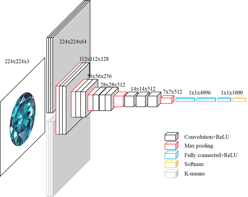
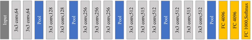
There are a total of four convolutional layers in the model frame. The first convolutional layer is called the data feature fusion layer, which fully fuses the denoising depth convolution and the main color feature. This is followed by a pooling layer whose role is to reduce network parameters and speed up fusion. The second convolutional layer is called the deep feature fusion layer, which undergoes further feature fusion, followed by a pooling layer. The third convolutional layer is called the feature abstraction representation layer, and the size of the convolutional kernel in this layer is changed from 5×5 in the first two convolutional layers to 3×3, which helps to eliminate noise in the feature and improve the abstract representation of the feature, followed by a pooling layer. The fourth convolutional layer, called the feature advanced presentation layer, helps eliminate redundant features and improve representative features, followed by a pooling layer. Three-layer fully connected layer for feature classification and parameter optimization during backpropagation. At the end of the network, the Softmax layer is used for clas- sification. Softmax is a supervised learning method for multi-classification problems [33, 34] that provides important confidence levels for classification, where 0 indicates the lowest confidence and 1 indicates the highest.

3.1. The k-means++ clustering algorithm extracts the dominant color features

The k-means++ clustering algorithm is a ’hard clustering’ algorithm, in which each sample in a dataset is scored 100% into a category. In contrast, ’soft clustering’ can be understood as a certain probability that each sample is sorted into a certain category.

The original k-means algorithminitially randomly selects k points in the dataset as cluster centers, while k-means++ selects 𝑘 cluster centers according to the following idea: assuming that n initial cluster centers have been selected.

The k-means++ clustering algorithm [35] is described as follows:

1. Randomly select a sample from the dataset as the initial cluster center 𝑐𝑖 .
2. First calculate the shortest distance between each sample and the current existing cluster center (that is, the distance from the nearest cluster center), expressed in terms of representation 𝐷 ( 𝑥 ); The probability that each sample will be chosen as the next cluster center is then calculated \(\frac{(D(x))^2}{\sum_{x \in X} (D(x))^2}\). Finally, the next cluster center is selected according to the roulette method.
3. Repeat Step 2 until a common cluster center 𝑘 is selected.
4. For each sample 𝑥( 𝑖) in the dataset, calculate its distance to a cluster center 𝑘 and divide it into classes corresponding to the cluster center with the smallest distance.
5. For each category 𝑐( 𝑖), recalculate its cluster center \(c_i = \frac{1}{|c_i|} \sum_{x \in c_i} X\) (i.e. the centroid of all samples belonging to that class).
6. Repeat Steps 4 and Step 5 until the position of the cluster center no longer changes.

3.2. Deep multi-feature fusion

Convolutional layers, nonlinearly activated transformations, and pooled layers are the three basic components of CNNs. By superimposing multiple convolutional layers with nonlinear operations and multiple pooling layers, a deep CNNs can be formed, which extract input features in layers, with invariance and robustness [36]. With specific architectures, such as local connections and shared weights, CNNs tend to have good generalization capabilities. Convolutional layers with nonlinear operations [32] are as follows (1):

$$x_j^l = f\left( \sum_{i=1}^{M} x_i^{l-1} * k_{ij}^l + b_j^l \right)\tag{1}$$

Where the matrix \(x_i^{l-1}\) is the ith feature map of the 𝑙 − 1 layer, \(x_j^{l}\) is the 𝑗th feature map of the current layer 𝑙, and 𝑀 is the number of input feature maps. \(k_l^{ij}\) and \(b_j^{l}\) are randomly initialized and set to zero, then fine-tuned precisely by backpropagation. 𝑓 ( · ) is a nonlinear activation function, and ∗ is a convolution operation.

The denoising depth convolution features 𝑓_𝑐 of the network structure output and the main color features extracted by the k-means++ clustering algorithm 𝑓_𝑙 are constructed according to the cascading and features of (2) to construct the deep integration features 𝑓_𝑚.

$$f_m = \alpha f_c + \beta f_l \tag{2}$$

Due to the high characteristic dimensions and limited training samples, overfitting is a serious problem that can occur. To solve this problem, the Dropout [37] method was used, which is a method of randomly deleting neurons during learning in Figure 2. During training, every time the data is passed, the neurons in the hidden layer are randomly selected, and then deleted, and the deleted neurons no longer transmit signals; During the test, although all neuronal signals are transmitted, the output of each neuron is multiplied by the deletion ratio at the time of training before the output. Therefore, the deleted neurons are not involved in forward transmission and are no longer used in the backward propagation process. At different training stages, deep networks form different neural networks by randomly discarding neurons. The Dropout method prevents complex co-adaptations, and neurons can learn more correct features.

4. Experiment

4.1. Datasets

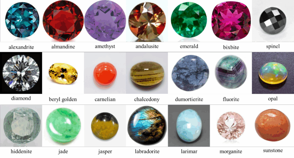
To verify the model orientation in this paper, a dataset of gemstone images obtained from [38] was selected for analysis. The dataset contains more than 3,200 images of different gemstone. The images are divided into 87 categories, which have been divided into training data and test data. Some of these examples are shown in Figure 3. Images are obtained under very different lighting and background color condi- tions. A total of 2800 images were used for training and 400 images were reserved for testing. For each class, there are 24-44 training images and 4-5 test images available.

The Epoch of the CNNs network model with deep multi- feature fusion is set to 50, the number of iterations is 8, and the batch size is 1000 images. The convolutional kernel size of the first convolutional layer is 5 *5, and the filter is 32; The convolutional kernel size of the second convolutional layer is 5*5, and the filter is 64; The convolutional kernel size of the third and fourth convolutional layers is 3*3, and the filter is 128. The convolution step is set to 1 and the fill is set to 0. The pooling layer step size is set to 2, and the pooling window size is 2*2. Finally, the Softmax layer has 10 neural units, indicating that the images are divided into 10 classes.

The optimal solution is obtained by minimizing the loss function. This study uses the cross-entropy error function [14] as the loss function, which is expressed as (3):

$$Q = -\frac{1}{N} \sum_{n=1}^{N} \left( (y_n \log_2(o_n) + \tilde{y}_n \log_2(\tilde{o}_n)) \right) \tag{3}$$

Where the \(\tilde{y}_n = 1 – y_n, \quad \tilde{o}_n = 1 – o_n\), Nnumber of samples is trained for batch processing, 𝑦 is the true label value for each sample, and 𝑜 is the actual output value of the network. 

To optimize the loss function, an optimization method is required, and the Adam optimizer is used for the experiment [15]. Combine the advantages of two optimization algorithms, AdaGrad and RMSProp. Considering the firstorder moment estimation (the mean of the gradient) and the second-order moment estimation (the undercentric variance of the gradient) of the gradient, the update step is calculated.

4.2. Experimental results and analysis

4.2.1. Evaluation function

To evaluate the performance of the algorithm, this paper uses a training validation test scheme in which 80% of the data is used as the training set and 20% as the test set. The test accuracy rate is used to evaluate the performance of the model and is expressed as (4):

$$Accuracy = \frac{R}{T} \tag{4}$$

where: 𝑅 is the sample with the correct classification and 𝑇 is the total sample.

4.2.2. Experimental results

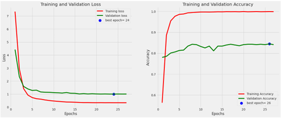
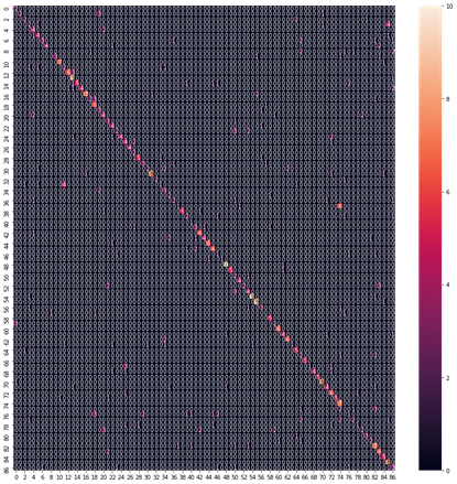
In this study, a convolutional neural network that deeply integrates the main color features with position and shape- related features, referred to as MCNN+. The model training results of MCNN+ are shown in the following Figure 4 and Figure 5. As can be seen from the Figure 4, the model gradually reaches a steady state after iterative training. One of the best classifications has an accuracy rate of 82%.

4.2.3. Model Comparison

We also compares the MCNN+ model with several machine learning models and deep learning models, as shown in the following Table 1.

Table 1: Comparison of different model results

As can be seen from the table, the model in this paper can achieve the best classification results when classifying the gemstone image data set. And it can be improved by nearly 9% compared to the CNN model.

5. Conclusion

In this study, we proposed a CNN gemstone image classification algorithm with deep multi-feature fusion, which effectively integrates the main color characteristics of gemstone images with the spatial position and shape characteristics extracted by convolutional neural networks. This approach addresses the limitation of traditional CNN models, which primarily focus on spatial position information and are less sensitive to color information. Experimental results demonstrate that MCNN+ not only significantly improves image classification performance but also exhibits greater stability and robustness. Additionally, our experiments show that different weight values in the MCNN+ network models have varying effects on experimental performance.

In future research, we aim to implement adaptive weight mechanisms to further enhance the model’s performance. Additionally, we plan to explore the integration of other feature extraction techniques, such as texture and edge detection, to enrich the feature set used for classification. We will also investigate the application of this model to other types of images and domains to test its versatility and generalizability. Finally, leveraging advanced techniques like transfer learning and self-supervised learning could further optimize the model and reduce the reliance on large labeled datasets.

Conflict of Interest The authors declare no conflict of interest.

Acknowledgment College of Jewelry, Shanghai Jian Qiao University.

1. D. Bersani, P. P. Lottici, “Applications of raman spectroscopy to gemol- ogy”, Analytical and bioanalytical chemistry, vol. 397, pp. 2631–2646, 2010, doi:10.1007/s00216-010-3700-1.
2. J. E. Shigley, “A review of current challenges for the identification of gemstones”, Geologija, , no. 64, 2008, doi:10.2478/v10056-008-0048-8.
3. L. Alzubaidi, J. Zhang, A. J. Humaidi, A. Al-Dujaili, Y. Duan, O. Al- Shamma, J. Santamaría, M. A. Fadhel, M. Al-Amidie, L. Farhan, “Review of deep learning: concepts, cnn architectures, challenges, applications, future directions”, Journal of big Data, vol. 8, pp. 1–74, 2021, doi:10.1186/s40537-021-00444-8.
4. T. Kattenborn, J. Leitloff, F. Schiefer, S. Hinz, “Review on convolu- tional neural networks (cnn) in vegetation remote sensing”, ISPRS journal of photogrammetry and remote sensing, vol. 173, pp. 24–49, 2021, doi:10.1016/j.isprsjprs.2020.12.010.
5. H. Gupta, K. H. Jin, H. Q. Nguyen, M. T. McCann, M. Unser, “Cnn- based projected gradient descent for consistent ct image reconstruc- tion”, IEEE transactions on medical imaging, vol. 37, no. 6, pp. 1440–1453, 2018, doi:10.1109/TMI.2018.2832656.
6. H. Lee, H. Kwon, “Going deeper with contextual cnn for hyperspectral image classification”, IEEE Transactions on Image Processing, vol. 26, no. 10, pp. 4843–4855, 2017, doi:10.1109/TIP.2017.2725580.
7. I. Maula, V. Amrizal, A. H. Setianingrum, N. Hakiem, “Develop- ment of a gemstone type identification system based on hsv space colour using an artificial neural network back propagation algorithm”, “International Conference on Science and Technology (ICOSAT 2017)- Promoting Sustainable Agriculture, Food Security, Energy, and En- vironment Through Science and Technology for Development”, pp. 104–109, Atlantis Press, 2017, doi:10.2991/icosat-17.2018.24.
8. A. Ostreika, M. Pivoras, A. Misevičius, T. Skersys, L. Paulauskas, “Clas- sification of objects by shape applied to amber gemstone classification”, Applied Sciences, vol. 11, no. 3, p. 1024, 2021, doi:10.3390/app11031024.
9. A. Ostreika, M. Pivoras, A. Misevičius, T. Skersys, L. Paulauskas, “Classification of amber gemstone objects by shape”, 2020, doi:10.20944/preprints202008.0336.v1.
10. R. S. Castro Rios, “Researching of the deep neural network for amber gemstone classification”, Master’s thesis, Universitat Politècnica de Catalunya, 2018.
11. S. Sinkevičius, A. Lipnickas, K. Rimkus, “Multiclass amber gemstones classification with various segmentation and committee strategies”, “2013 IEEE 7th International Conference on Intelligent Data Acqui- sition and Advanced Computing Systems (IDAACS)”, vol. 1, pp. 304–308, IEEE, 2013, doi:10.1109/IDAACS.2013.6662694.
12. X. Liu, J. Mao, “Research on key technology of diamond particle detection based on machine vision”, “MATEC Web of Conferences”, vol. 232, p. 02059, EDP Sciences, 2018, doi:10.1051/matecconf/201823202059.
13. B. H. Y. Chow, C. C. Reyes-Aldasoro, “Automatic gemstone classifi- cation using computer vision”, Minerals, vol. 12, no. 1, p. 60, 2021, doi:10.3390/min12010060.
14. K. Hurrell, M. L. Johnson, Gemstones: a complete color reference for precious and semiprecious stones of the world, Chartwell Books, 2016.
15. C. M. Breeding, A. H. Shen, S. Eaton-Magaña, G. R. Rossman, J. E. Shigley, A. Gilbertson, “Developments in gemstone analysis tech- niques and instrumentation during the 2000s.”, Gems & Gemology, vol. 46, no. 3, 2010.
16. R. Liddicoat, “Developing the powers of observation in gem testing”, Gems Gemol, vol. 10, pp. 291–319, 1962.
17. E. Fritsch, C. M. Stockton, “Infrared spectroscopy in gem identifica- tion”, Gems & gemology, vol. 23, no. 1, pp. 18–26, 1987.
18. A. L. Jenkins, R. A. Larsen, “Gemstone identification using raman spectroscopy”, disclosure, vol. 7, p. 9, 2004.
19. L. Kiefert, S. Karampelas, “Use of the raman spectrometer in gemmological laboratories”, Spectrochimica Acta Part A: Molecular and Biomolecular Spectroscopy, vol. 80, no. 1, pp. 119–124, 2011, doi:10.1016/j.saa.2011.03.004.
20. T. He, “The applications of ultraviolet visible absorption spectrum detection technology in gemstone identification”, “Proceedings of the 5th International Conference on Materials Engineering for Advanced Technologies (ICMEAT 2016), Quebec, QC, Canada”, pp. 5–6, 2016.
21. S. Thompson, F. Fueten, D. Bockus, “Mineral identification using artificial neural networks and the rotating polarizer stage”, Computers & Geosciences, vol. 27, no. 9, pp. 1081–1089, 2001, doi:10.1016/S0098- 3004(00)00153-9.
22. N. A. Baykan, N. Yılmaz, “Mineral identification using color spaces and artificial neural networks”, Computers & Geosciences, vol. 36, no. 1, pp. 91–97, 2010, doi:10.1016/j.cageo.2009.04.009.
23. H. Izadi, J. Sadri, M. Bayati, “An intelligent system for mineral identi- fication in thin sections based on a cascade approach”, Computers & Geosciences, vol. 99, pp. 37–49, 2017, doi:10.1016/j.cageo.2016.10.010.
24. H. Pereira Borges, M. S. de Aguiar, “Mineral classification using machine learning and images of microscopic rock thin section”, “Advances in Soft Computing: 18th Mexican International Confer- ence on Artificial Intelligence, MICAI 2019, Xalapa, Mexico, October 27–November 2, 2019, Proceedings 18”, pp. 63–76, Springer, 2019, doi:10.1007/978-3-030-33749-0_6.
25. J. Maitre, K. Bouchard, L. P. Bédard, “Mineral grains recognition using computer vision and machine learning”, Computers & Geosciences, vol. 130, pp. 84–93, 2019, doi:10.1016/j.cageo.2019.05.009.
26. Y. Zhang, M. Li, S. Han, Q. Ren, J. Shi, “Intelligent identifi- cation for rock-mineral microscopic images using ensemble ma- chine learning algorithms”, Sensors, vol. 19, no. 18, p. 3914, 2019, doi:10.3390/s19183914.
27. K. Muthukaruppan, S. Thirugnanam, R. Nagarajan, M. Rizon, S. Yaa- cob, M. Muthukumaran, T. Ramachandran, “A comparison of south east asian face emotion classification based on optimized ellipse data using clustering technique”, Journal of Image and Graphics, vol. 3, no. 1, 2015, doi:https://doi.org/10.18178/joig.3.1.1-5.
28. Y. Karayaneva, D. Hintea, “Object recognition in python and mnist dataset modification and recognition with five machine learning classifiers”, Journal of Image and Graphics, vol. 6, no. 1, pp. 10–20, 2018.
29. L. Wang, B. Liu, S. Xu, J. Pan, Q. Zhou, “Ai auxiliary labeling and clas- sification of breast ultrasound images”, Journal of Image and Graphics, vol. 9, no. 2, pp. 45–49, 2021.
30. N. M. Trieu, N. T. Thinh, “A study of combining knn and ann for classifying dragon fruits automatically”, Journal of Image and Graphics, vol. 10, no. 1, pp. 28–35, 2022.
31. J. Gu, Z. Wang, J. Kuen, L. Ma, A. Shahroudy, B. Shuai, T. Liu,
    X. Wang, G. Wang, J. Cai, et al., “Recent advances in convolutional neural networks”, Pattern recognition, vol. 77, pp. 354–377, 2018, doi:10.1016/j.patcog.2017.10.013.
32. Y. Chen, C. Li, P. Ghamisi, X. Jia, Y. Gu, “Deep fusion of re- mote sensing data for accurate classification”, IEEE Geoscience and Remote Sensing Letters, vol. 14, no. 8, pp. 1253–1257, 2017, doi:10.1109/LGRS.2017.2704625.
33. R. Kiran, P. Kumar, B. Bhasker, “Dnnrec: A novel deep learning based hybrid recommender system”, Expert Systems with Applications, vol. 144, p. 113054, 2020, doi:10.1016/j.eswa.2019.113054.
34. X. Peng, X. Zhang, Y. Li, B. Liu, “Research on image feature extraction and retrieval algorithms based on convolutional neural network”, Journal of Visual Communication and Image Representation, vol. 69, p. 102705, 2020, doi:10.1016/j.jvcir.2019.102705.
35. D. Arthur, S. Vassilvitskii, “k-means++: The advantages of careful seeding”, Tech. rep., Stanford, 2006.
36. Y. Bengio, A. Courville, P. Vincent, “Representation learning: A review and new perspectives”, IEEE transactions on pattern anal- ysis and machine intelligence, vol. 35, no. 8, pp. 1798–1828, 2013, doi:10.1109/TPAMI.2013.50.
37. D. Steinkraus, I. Buck, P. Y. Simard, “Using gpus for machine learn- ing algorithms”, “Eighth International Conference on Document Analysis and Recognition (ICDAR’05)”, pp. 1115–1120, IEEE, 2005, doi:10.1109/ICDAR.2005.251.
38. “Gemstone images”, https://www.kaggle.com/lsind18/ gemstone-images.

Citations by Dimensions

Citations by PlumX

Crossref Citations

This paper is currently not cited.

No. of Downloads per Month

No. of Downloads per Country