Imbalanced dataset handling in real time is one of the most challenging tasks in predictive modelling. This work handles the critical issues arising in imbalanced dataset with implementation of artificial neural network and deep neural network architecture. The usual machine learning algorithms fails to achieve desired throughput with certain input circumstances due to mismatched class ratios in the sample dataset. Dealing with imbalanced dataset leads to performance degradation and interpretability issue in traditional ML architectures. For regression tasks, where the target variable is continuous, the skewed data distribution is major issue. In this study, we have investigated a detailed comparison of traditional ML algorithms and neural networks with dimensionality reduction method to overcome this problem. Principle component analysis has been used for feature selection and analysis on real time satellite-based air pollution dataset. Five regression algorithms Multilinear, Ridge, Lasso, Elastic Net and SVM regression is combined with PCA and non PCA to interpret the outcome. To address unbalanced datasets in real-time, deep neural networks and artificial neural network architectures have been developed. Each model’s experiments and mathematical modelling is done independently. The Deep neural network is superior compared to other conventional models for performance measures of target variable in imbalanced datasets.

1. Introduction

In the domain of artificial intelligence (AI), the persistent challenge of imbalanced datasets remains a focal point. Accuracy, a prime indicator of model performance is primarily dependent on the balance of the data set. This issue is of paramount importance in practical applications like fraud detection [1], medical diagnosis [2], remote sensing [3], engineering [4] and anomaly detection [5], where the class of interest is typically a minority within the dataset. An uneven distribution of inputs and outputs (classes) in an imbalanced dataset is defined as one class, called the minority class, having substantially fewer instances than the other classes, called the majority class. Due to the uneven class ratios in the dataset, handling unbalanced datasets presents a challenge. In an out of balanced dataset, the majority class may make up a large portion of the training dataset, while the minority class is underrepresented in the dataset. The problem with a model trained on such out of balanced data set is that the model progressively learns to achieve high accuracy by consistently predicting the majority class, even if recognizing the minority class is equal or more important when applying the model to a real-world scenario.

Many machine learning approaches have been widely applied in a variety of applications. Machine learning models such as Multilinear Regression (MLR), Ridge Regression (RR), Lasso Regression (LR) and Elastic Net Regression (ELR) are mainly used for regression task in diverse ways. However, the traditional regression algorithms are not always beneficial to meet the requirement of large-scale raw datasets.

One of the most helpful algorithms that aims to identify underlying links in a batch of data by simulating how the human brain functions is the neural network. Neural networks are one of the most effective methods for fitting various types of stationary and non-stationary data. A degree of balance in the dataset is essential for neural networks to function well. However, the conventional assumption of a balanced data becomes untenable for certain scenarios, where the minority class is significantly underrepresented. This imbalance leads neural networks to exhibit negative performance, particularly in accurate prediction of minority classes. The issue of data imbalance can also be addressed via deep learning synaptic models, which have been shown to considerably raise performance benchmarks in both regression and classification tasks. Neural networks topologies keep changing and getting better in 21st century, that present an opportunity to enhance the computational modeling capabilities and enabling more accurate predictions in various data-driven use cases [6].

1.1. Hypothesis

In an imbalanced stationary dataset, the neural network-based architecture works more efficiently and produce better performance accuracy over multiple regression models (MLR, RR, LR, ELR).

1.2. Objective

This research implements a novel way to apply neural networks to imbalanced real-time satellite datasets. Multiple regression model is trained for analyzing the performance for real time satellite data based on Air Quality Index (AQI) prediction. The same dataset is used for the implementation of Multilinear Regression (MLR), Ridge Regression (RR), Lasso Regression (LR), Elastic Net Regression (ELR), and Support Vector Machine Regression (SVM). In addition, the dataset is processed using Principal Component Analysis (PCA). Essentially, two neural network architectures- the Artificial Neural Network (ANN) and the Deep Neural Network (DNN) are compared with four traditional regression models and SVM. After comparison, the proposed method produced promising results which shows how to analyze the imbalanced dataset in an effective manner. Experiments are presented to demonstrate how the neural network approach efficiently improves the model accuracy and R- squared score (R2).

2. Literature Review

 Earlier works which specified different approaches and methods for theoretical and practical implementation as well as handling the imbalanced dataset are discussed below:

A training procedure for Multilayer Perceptron (MLPs) is implemented using an imbalanced dataset. This article [3] uses a remote-sensing dataset that includes agricultural classes including potatoes, carrots, wheat, sugar beets, and stubble. The suggested method seeks to increase the stability of classification findings and accelerate training by an average of 41.5 times.

In order to solve Haberman’s surviving unbalanced data set challenges, a modified learning method [6] for ANN is presented. The artificial neural network’s output layer uses Particle Swarm Optimization (PSO) as part of its technique to optimize the step function’s decision boundary. The study demonstrates increase in the average Geometric-Mean Test of classifier performance (80.16 for training and 70.47 for testing).

Three image data sets and five document data sets with different degrees of imbalance are used in an experiment [7]. It proposed a loss function called mean false error (MFE) and its enhanced counterpart, mean squared false error (MSFE), for training DNN on unbalanced data sets. Theoretical analysis is empirically confirmed, and experiments and comparisons demonstrating the superiority of the proposed approach over traditional methods in classifying imbalanced data sets on deep neural networks demonstrate the effectiveness of the proposed methods in extremely imbalanced data sets.

The creation of a system to simulate and predict maize and soybean yields on a county-by-county basis in the American Midwest and Great Plains using Artificial Neural Networks (ANN) has been studied [8]. It utilized multi-temporal remote sensing images to derive NDVI values, which characterized the entire growing process. The methodology employed a feed-forward multi-layer perceptron (MLP) neural network for learning and the SCE-UA method for training the NN. The outcomes showed that multivariate linear regression (MLR) is 20% inferior than the ANN.

The purpose of gathering seven severely unbalanced data sets [9] is to assess how well various Support Vector Machine (SVM) modelling techniques work. Various “rebalance” procedures, including cost-sensitive learning and over and under sampling, were included into SVM modelling to tackle the problem of class imbalance. It introduced GSVM-RU algorithm, which comes up as a state of art approach with 85.2 G-Mean, 91.4 AUC- ROC, 66.5 F Measure and 181 Efficiency.

The work [10] focuses on the unique problem of Deep Imbalanced Regression (DIR) and uses large-scale datasets from computer vision, natural language processing, and healthcare. Feature distribution smoothing (FDS) and label distribution smoothing (LDS) are two efficient techniques that the study suggests using to handle unbalanced data with continuous objectives. The MAE and G-Mean improved significantly ranged from 0.1 to 2.7.

A large-scale dataset is utilized including face attribute classification and edge detection tasks, as well as controlled class imbalance in the MNIST digit classification. A novel method [11] for learning deep feature embeddings that effectively handle imbalanced data classification. The proposed approach involves quintuplet sampling and a triple-header hinge loss to enforce relationships during feature learning. The LMLE- kNN has outperformed by a large margin with a mean per class accuracy of 84 as compared to other traditional method.

To confirm the notion that models trained using Dense Loss perform better in underrepresented areas of the dataset than models built with a conventional training approach, synthetic datasets [12] with varied features, such as heavy-tailed datasets, are utilized. The findings demonstrated that MLP with Dense Loss performs better than MLP without Dense Loss, with an average Root Mean Square Value (RMSE) ranging from 1.21 to 7.02.

According to a study [13] on small and medium-sized enterprises (SMEs) in Malaysia, such as those in the transportation, storage, catering, lodging, and hotel industries, the Synthetic Minority Oversampling Technique (SMOTE) is effective in improving the classification accuracy of logistic regression models when the data are highly unbalanced. The study used a dataset of 601 failed and 26,284 failing SMEs between 1999 and 2013. The findings demonstrated that, with 57.23% sensitivity and 58.83% specificity, the SMOTE logistic regression technique produced superior metrics when compared to classical logistic regression.

SMOGN algorithm [14] combines two oversampling techniques knows as SMOTE and gaussian noise. This algorithm is used as a preprocessing solution for unbalanced regression problems with the aim of improving the performance of regression algorithms. SMOGN performs exceptionally well with multivariate adaptive regression spline (MARS) and random forest (RF) learners, demonstrating enhanced recall without appreciable loss of precision, according to tests on 20 distinct regression datasets.

3. Materials and Methods

This section introduces the imbalanced stationary data regression algorithms and the experimental data sets used in this study.

3.1. Dataset

The dataset consists of the satellite records of greenhouse gases (GHGs) emission in India. The initial dataset consists of two million five hundred eighty nine thousand and eighty three sets of reviews. It possesses a total of fifteen features as Stationid, PM2.5, PM10, NO, NO2, NOx, NH3, CO, SO2, O3, Benzene, Toluene, Xylene, AQI and AQI_Bucket. The raw data belongs to a stationary imbalanced category. A preprocessed version of the data having five thousand and ninety two samples is utilized in this study. The dataset used in this study contains no missing features. The original dataset is open source and can be downloaded here: https://www.kaggle.com/datasets/rohanrao/air-quality- data-in-india?select=station_hour.csv

3.2. Operating system and software

The analytical code implementation and execution have been conducted on a 64-bit operating system with an x64-based processor system type, complemented by 8GB of RAM. Version 6.3.0 of Jupyter Notebook is utilized as an interactive programming environment. In addition, the Python script has been run on the Google Colab cloud platform, which has an Intel(R) Xeon(R) CPU operating at 2.30 GHz, 12.7 GB of RAM, and 108 GB of disc space.

3.3. Data Preprocessing

The quality of the underlying data is the primary determinant of the success of visualizations and the construction of efficient machine learning (ML) models. Preprocessing is essential for increasing data quality since it reduces noise, which boosts ML systems’ processing speed and capacity for generalization. Two prevalent issues encountered in data extraction and monitoring applications are outliers and missing data. Different techniques have been employed to identify outlier values and handle not-a-number (NAN) values. Table 1 shows the visual representation of distribution of missing values across different features of the dataset. Notably, Xylene emerges as the feature with the highest number of missing values, while CO exhibits the least. To guarantee that the significance of the variables is not impacted by changes in their ranges or units, all missing values have been removed from the dataset and the standard scaler normalization process has been executed.

Table 1: Missing Values of Features.

3.4.  Feature Selection

To select significant features, the correlation of the AQI with other features has been analyzed. Table 2 displays the precise correlation values between the AQI and each contaminant in the dataset. It is evident that the majority of the features have very little correlation. The ideal number of input variables for the creation of machine learning models has been found using a feature selection method based on Principle Component Analysis (PCA). To improve computing efficiency and accuracy, the intended objective is to project a d-dimensional dataset onto a (k)-dimensional subspace in order to minimize its dimensions.

Table 2: Correlation between AQI and Pollutants.

3.5. Experiment Performed

 3.5.1.  Proposed Architecture

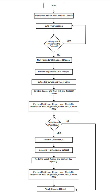
Figure 1 illustrates the workflow of our proposed architecture. It begins with collecting dataset and data preprocessing. After that, it checks if there are any missing values present or not in the dataset. It there are no missing values then the non-redundant dataset go through the exploratory data analysis process. The next steps involve applying the features and target value into various ML and neural network architecture. If the result is unstable, and poor then the input goes through PCA with 2, 3 and 5 components to enhance the model stability and handle the imbalanced real time dataset. After PCA, it selects the optimal features and target values to perform data splitting and perform regression to produce the improved results. This approach enhanced the model stability, interpretability and able to overcome the issue of handling imbalanced dataset using standard regression models.

3.6. Algorithm

Algorithm: PCA Combined Neural Network

Input: D → Complete dataset (Station hour Satellite dataset)

Output: Predicted AQI Value

3.7. Steps

1) Load and Clean Data

Load Dataset D, handle missing values and make the dataset non-redundant.

2) Perform Initial EDA and Model Evaluation

• Define features and target
• Split dataset into training (80%) and testing (20%)
• Apply the following 7 models on the imbalanced dataset: MLR, RR, LR, ELR, SVM, Vanilla ANN and Custom DNN
• Evaluate performance metrics and check if the results are unstable or not. If the results are not good then go to step 3.

3) Apply Custom PCA

• Standardize the dataset: 𝑋𝑠𝑡𝑑 = 𝑋 − 𝜇/𝜎 , where 𝑋 is the original data, 𝜇 is the mean and 𝜎 is the standard deviation statistical error that separates an observation from its predicted
• Compute Covariance Matrix: \(\Sigma = \frac{1}{n – 1} X_{std}^T X_{std}\) , where Σ is the covariance matrix, \(X_{std}^T\) is the transpose of the standardized data, and n is the number of observations.
• Obtain Eigenvectors and Eigenvalues: 𝛴v=𝜆v , , where v is the eigenvectors and 𝜆 is the eigenvalues.
• Select Top 𝑘 Eigenvectors: Sort eigenvalues in descending order and select the top 𝑘 eigenvectors corresponding to the largest eigenvalues. Construct the projection matrix 𝑊 from these eigenvectors.
• Transform Data: 𝑌=𝑋_𝑠td𝑊 , Where 𝑌 is the transformed data in the new 𝑘-dimensional space.

4) Perform Regression with PCA optimized data:

• Split PCA-transformed data into training (80%) and testing (20%) sets.
• Apply the following 7 models in the dataset 𝑌 with 2 component PCA, 3 component PCA and 5 component PCA: MLR, RR, LR, ELR, SVM, Vanilla ANN and Custom DNN
• Evaluate performance for each configuration

5) Compare Results: Compare performance metrics from initial and PCA-transformed datasets to get the improved

3.7.1. Proposed Model

For this work, five regression model, and two neural network-based architecture models are introduced.

3.7.1.1. Multilinear Regression

Multilinear regression (MLR) is an analytical method of predicting the value of a specific metric by taking into account several independent variables. This algorithm is used to find the optimal straight line to predict the AQI value for various parameters. First, we define the independent features as x1, x2, ………., x10. Then, we have defined the dependent feature as y i.e., AQI. It can be mathematically represented via equation 1.
$$y = \beta_0 + \beta_1 x_1 + \beta_2 x_2 + \cdots + \beta_n x_n + \epsilon \tag{1}$$

For nth observation, 𝛽₀ is a constant term also known as y-intercept and 𝛽𝑛 is the slope coefficient for each explanatory variable. Parameter 𝜖 stands for the statistical error that separates an observation from its predicted value.

3.7.1.2. Ridge, Lasso and Elastic Net Regression

It is common for real-time unbalanced datasets to have a significantly larger number of input variables than observations. With many predictors, fitting the full model without penalization will result in large prediction intervals. For that reason, we have used three model tuning regression method i.e., Ridge Regression (RR), Lasso Regression (LR) and Elastic Net Regression (ELR) to analyze the problem better. RR constitutes a model refinement technique employed for the analysis of datasets afflicted by multicollinearity [15]. Employing L2 regularization, this method addresses situations where the occurrence of multicollinearity imparts bias to least-squares estimates and induces elevated variances. The mathematical representation of RR is in equation 2.

$$RRL_2 = \sum_{i=1}^{n} (y_i – \hat{y}_i)^2 + \lambda \sum_{j=1}^{P} \beta_j^2 \tag{2}$$

Here, the L2 term is equivalent to the square of the coefficient magnitudes (j) and the regularisation penalty is denoted by . As we increase the value of  this constraint causes the value of the coefficient to tend towards zero [16]. By applying a penalty proportional to the absolute value of the magnitude of the coefficients, Lasso regression carries out L1 regularisation (equation 3). Certain coefficients may become zero and be removed from the model as a result of this kind of regularisation, producing sparse models with few coefficients.

$$LRL_1 = \sum_{i=1}^{n} (y_i – \hat{y}_i)^2 + \lambda \sum_{j=1}^{P} |\beta_j| \tag{3}$$

To improve the model prediction rate, both regularization of lasso and ridge are combined to produce the elastic net model loss. The collinearity coefficient is difficult to eradicate, according to the fundamental rationale behind. In this study, the Grid Search approach (GS) for hyperparameter tweaking has been employed to enhance the model’s performance. This research makes use of the Scikit-Learn class GridSearchCV. The GridSearchCV evaluates, all possible combinations of parameter values and finally, the best parameter combination is retained. After tuning the optimal 𝜆 value is 1, 0.0001, and 0.0001, for RR, LR, and ELR, respectively.

3.7.1.3. Support Vector Machine (SVM)

SVM divides data into multiple classes by locating a hyperplane in a high-dimensional space [17]. The primary objective is to optimize the margin, which is the space between the hyperplane and the closest support vectors, while simultaneously minimizing the error SVM uses a technique called the kernel trick to translate the feature space into a higher-dimensional space in order to improve data point separation when dealing with non- linearly separable data [18], [19]. The kernel functions used in the SVM model are linear and Radial Basis Function (RBF). The hyperparameter C, and epsilon, are taken as 5, and 1, respectively after tuning for the proposed model. C is the regularization parameter that controls the trade-off between achieving a low training and testing error while maximizing the margin. Epsilon is the width of the epsilon-insensitive tube in SVM Regression. It defines a margin of tolerance where no penalty is given to errors.

3.7.1.4. Artificial Neural Network (ANN)

The best model for automatically identifying and simulating intricate non-linear correlations between the “output” (i.e. AQI) and the “inputs” (i.e. NO, NO2, NH3 etc.) of the network is the artificial neural network (ANN), which can also take into account all potential interactions between the input variables [20]. As imbalanced dataset contains a large proportions of skewed classes so conventional regression method fails to recognise the non- linear relationship between inputs and outputs. The architectural depiction of the ANN model employed in this study is displayed in Figure. 2.

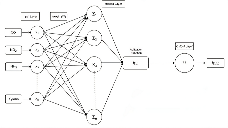
The ANN consists of one input, one hidden and one output layer. The input features are represented as X1, X2, X3,…., Xn. The synaptic weights between the input and hidden layer are defined as W1, W2,…Wn. The biases are taken as b0 and b1 for hidden and output layer respectively. Σ denotes each node takes the weighted sum of its inputs, and passes it through a non-linear activation function. The mathematical equation of tanh is represented via equation 4.

$$f(\Sigma) = \frac{e^x – e^{-x}}{e^x + e^{-x}} = \frac{1 – e^{-2x}}{1 + e^{-2x}} \tag{4}$$

The AQI value is then predicted by feeding the hidden layer’s output into the output layer. To reduce the error rate during backpropagation, the gradient descent is calculated and used to modify the weights and biases. The ANN model has been analysed combined with PCA for 2, 3 and 5 components respectively to increase the model interpretability and computational efficiency.

3.7.1.5. Deep Neural Network (DNN)

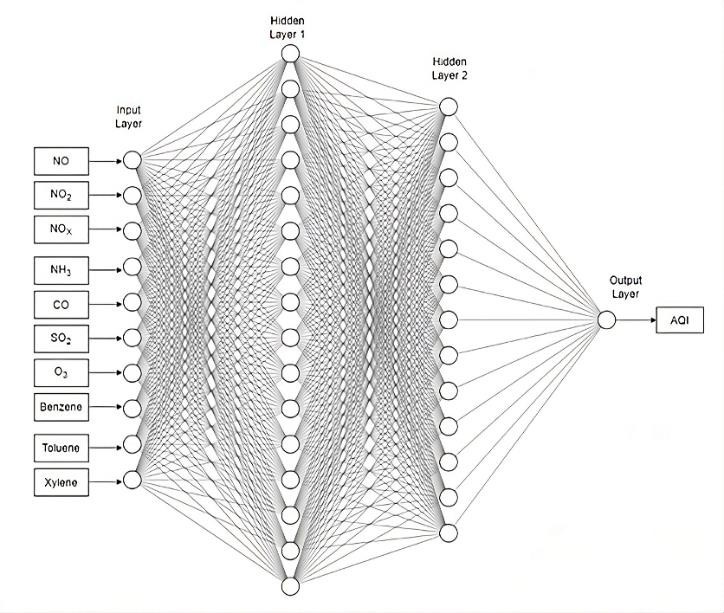
DNN refers to a multilayer perceptron model that has more than one hidden layer. When it comes to assessing the AQI value, DNN is a more potent and reliable neural network model than ANN. DNN exhibits of layer wise feature extraction methodology and combine low level feature to generate high level features [21], [22]. Figure. 3 shows the visual representation of DNN model. It is composed of one input layer with 10 neurons, two hidden layer (i.e., 256 and 512 neurons respectively) and one output layer. Weights and biases are initialised to the proper values at each layer of the network. Rectified Linear Unit (ReLu) activation function (represented by equation 5) and linear function are utilised at the hidden layer and output layer, respectively. To achieve state of the art performance, the model has then been evaluated using a combination of PCA and DNN.

ReLu (z) = max (0, z)                                 (5)

4. Results

The models for forecasting the AQI level based on different atmospheric pollution characteristics are empirically evaluated in this section. Metrics such as mean absolute error (MAE), mean squared error (MSE), root mean square error (RMSE), mean absolute percentage error (MAPE), and coefficient of determination (R2) have been used to evaluate the model. Every model has been simultaneously trained, examined, and integrated using PCA and non-PCA analysis. For RR, LR, ELR, and SVM regression, the Grid Search method has been used.

Table 3: Comparison of Regression model results without PCA.

The performance characteristics of a standard regression model with and without Principal Component Analysis (PCA) integration are shown in Tables 3 and 4, respectively. We can clearly see that RR has outperformed as compared to other model in terms of MSE and R2 score.

MLR and LR has slightly degraded performance in both normal and grid search method (GS) as compared to RR. After using PCA, it is shown that using five principal components produces outcomes that are almost similar to those that come from non-PCA analysis.

The association between the independent variables and AQI is explained in great detail by the trained MLR model. Equation 6 provides a statistical illustration of the concept represented in equation 1. Because LR regression employs the L1 norm, some of the coefficients are absolutely zero. This shows that the relevant elements have been effectively excluded from the model, rendering them useless in predicting the target variable. This increases model interpretability while also possibly improving prediction performance by decreasing overfitting.

$$\text{MLR}(Y_{AQI}) = [4.6,\ 27.41,\ -18.07,\ 10.84,\ 4.02,\ -0.21,\ 18.98,\\4.85,\ 1.61,\ -0.27]_{1 \times 10} \begin{bmatrix} X_1 \\ X_2 \\ \vdots \\ X_{10} \end{bmatrix}_{10 \times 1} + 92.57 \tag{6}$$

The equation 6 represents the coefficient matrix (𝛽₁ = 4.6, 𝛽₂ = 27.41, ……., 𝛽₁₀ =−0.27),, independent features from NO to Toluene (X1, X2,…,X10)and intercept value (𝛽₀ = 92.57) for MLR. The values from 𝛽₀ to 𝛽₁₀  are experimentally obtained corresponding to the MLR entry of table 3 without PCA. Similarly, equation 7, equation 8 and equation 9 defines the coefficient matrix, independent features and intercept values used for RR, LR and ELR model respectively. The statistical equations from 7 to 9 are generated with all the features without using PCA. The final combined PCA model equations along with coefficient matrix and intercept can also be generated in the similar way.

$$\text{RR}(Y_{AQI}) = [2.01,\ 21.07,\ -10.47,\ 10.87,\ 3.99,\ -0.19,\ 18.95,\ 4.81,\\ 1.62,\ -0.27]_{1 \times 10} \begin{bmatrix} X_1 \\ X_2 \\ \vdots \\ X_{10} \end{bmatrix}_{10 \times 1} + 92.57 \tag{7}$$

$$\text{LR}(Y_{AQI}) = [-1.47\text{e}{-02},\ 1.15\text{e}{+01},\ 0,\ 1.11\text{e}{+01},\ 3.28,\ 0,\\ 1.8\text{e}{+01},\ 4.46,\ 8.99\text{e}{-01},\ 0]_{1 \times 10} \begin{bmatrix} X_1 \\ X_2 \\ \vdots \\ X_{10} \end{bmatrix}_{10 \times 1} + 92.57 \tag{8}$$

$$\text{ELR}(Y_{AQI}) = [-1.41,\ 5.07,\ 3.23,\ 9.27,\ 4.36,\ 2.07,\ 12.3,\ 3.81,\ 2,\\ 0.97]_{1 \times 10} \begin{bmatrix} X_1 \\ X_2 \\ \vdots \\ X_{10} \end{bmatrix}_{10 \times 1} + 92.57 \tag{9}$$

As compared to traditional regression model SVM works better than in terms of R2 score. Table 5 describes that RBF with GS approach has the lowest RMSE and R2 score as compared to linear and normal RBF. With implementation of combined PCA and SVM, the model able to able to outperformed in each type of kernel by high margin. In regression, accuracy refers to the model’s ability to forecast the percentage difference between the actual and estimated values. Table 5 compares all three types of SVM kernels to determine the overall best accuracy.

The derived equations for the linear and RBF kernels are provided in equations 10 and 11, respectively. The results of the AQI prediction are obtained using these equations. For linear SVM, positive coefficients indicate that a factor has a positive effect on predicted AQI, while negative coefficients indicate a negative effect. The intercept term represents the baseline AQI value. In contrast, with the RBF-kernelized SVM, the dual coefficients indicate the importance of the support vector in defining the decision region, with positive and negative coefficients indicating the direction of the effect on the predicted AQI.

Table 4: Comparison of Regression Model results with PCA

Table 5: SVM Regression Results with PCA and NON PCA.

Table 6: Comparison of ANN Model Results.

After training using linear SVM equation 10 shows the final weight matrix (W1= -0.3, W2= 0.52,……, W10= 0.09), input feature matrix (X1, X2,…,X10) and bias as 9.58 for computing the AQI output. The RBF kernel based SVM represented via equation 11 analyze for the weights consisting between -1 and 1, bias term (113.14), input feature vectors from X1 to X10 and each support vectors () passing through X1 to X10.

F(AQI) = [-0.30, 0.52, 0.03, 1.99, 4.41, 0.21, 0.59, 1.28, 0.18,

$$[0.09]_{1 \times 10} \begin{bmatrix} X_1 \\ X_2 \\ \vdots \\ X_{10} \end{bmatrix}_{10 \times 1} + 9.58 \tag{10}$$

Table 6 shows the result after training the imbalanced dataset using ANN architecture. ANN outperformed all of the earlier models in terms of strength and performance. It achieved lowest RMSE and MSE as compared to SVM, RR, LR, ELR and  MLR. ANN  Model

Table 7: Comparison of DNN Network Results

obtained with ten inputs, one hidden layer with one twenty-eight neurons and final output layer with predicted AQI value.

$$f(\text{AQI}) = [-1,\ -1,\ -1,\ \ldots,\ 1,\ -1,\ 1]_{1 \times 10} \begin{bmatrix} K(X, X_1) \\ K(X, X_2) \\ \vdots \\ K(X, X_{10}) \end{bmatrix}_{10 \times 1} + 113.14 \tag{11}$$

The DNN Model is a very sophisticated and potent neural network designed to manage unbalanced datasets. Table 7 shows that the DNN model works better than the ANN by significantly increasing the R2 score and simultaneously decreasing metrics like MSE, MAE, and RMSE. Notably, the DNN model gets an accuracy rate of 82.78%, outperforming all other models in the comparison

A lower MSE and a higher R² score indicate that the DNN model also performs even better than conventional regression models. The DNN model is more successful without requiring feature extraction, as seen by its lower RMSE and greater accuracy when compared to the SVM model using five component PCA. During training, ANN and DNN possess the ability to autonomously extract meaningful features from raw data. They can adapt to high-dimensional input spaces without explicit feature extraction. ANN and DNN model with combined PCA result has been shown in table 6 and table 7 respectively. However, complicated connections among features can be handled by the proposed DNN model without the need for PCA. This not only increases efficiency and interpretability, but also reduces training time and computational cost, making the DNN model a state-of-the-art approach for various performance metrics

DNN model takes ten neuronal inputs, and two hidden layers consisting of two fifty-six and five hundred twelve neurons respectively. The output layer involves a 5121- dimensional weight matrix along with a linear function to derive the AQI value.

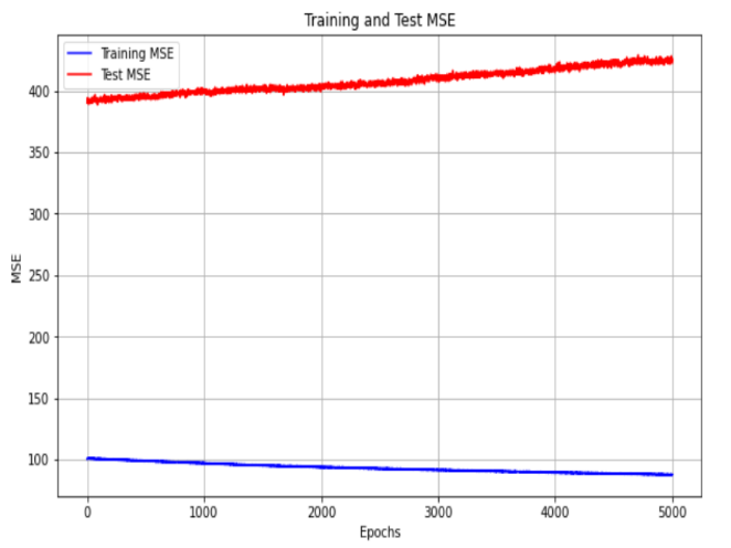
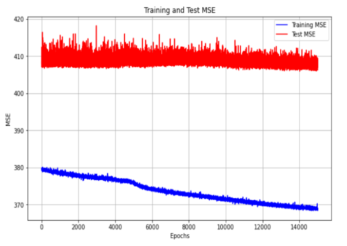
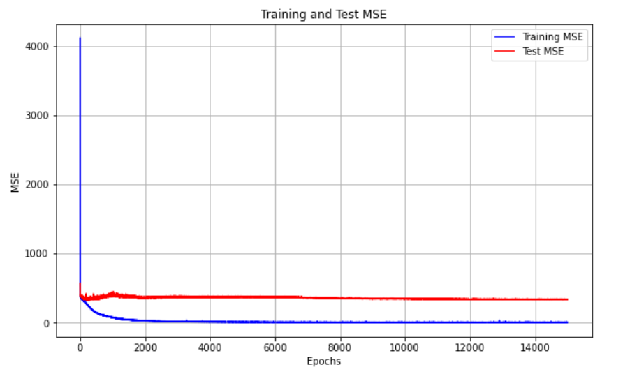
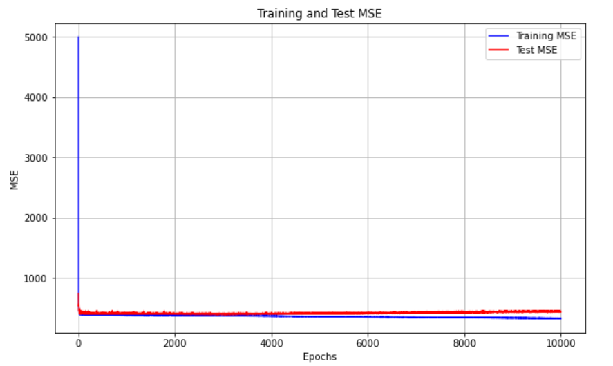
Figure 4 and 5 illustrate the rate of MSE change for the ANN model employing 10 input features and utilizing dimensionality reduction with 2 features, respectively. It is clear that the ANN model with 10 input features converges much more quickly than the one using 2 features plus PCA because of inadequate feature representation. Similarly, Figure 6 and 7 depict the MSE convergence dynamics during the training of neural network architectures for final output layer prediction. The DNN model exhibits standard MSE performance in both training and testing datasets, while the DNN utilizing 2 principal components tends to converge prematurely, resulting in less accurate predictions for the final output layer.

Consequently, our original DNN synaptic model architecture demonstrates superior performance with robust convergence compared to alternative networks.

DNN models can converge faster and produce more accurate results without the usage of PCA. The suggested DNN model is advantageous for achieving optimal outcomes, especially in scenarios involving imbalanced datasets.

PCA effectively reduces the dimensionality of the dataset into 2, 3, and 5 components, respectively. It identifies the most significant features by projecting the data into k-dimensional spaces that capture the most critical variance. This process streamlines the data, minimizing noise and redundancy, which makes the data more regular and structured. By introducing the most relevant components, PCA allows the DNN to operate more efficiently, avoiding overfitting and improving its ability to learn complex patterns in the data. This enhancement in data regularity enables the DNN to outperform other regression models in terms of performance and interpretability.

5. Conclusion

Though “Accuracy” is a prime indicator of model performance however its reliability depends upon the dataset. In an out of balanced dataset, the majority class makes up a large portion of the training dataset, while the minority class is underrepresented in the dataset. The problem with a model trained on this out of balanced data set is that the model learns that it can achieve high accuracy by consistently predicting the majority class, even if recognizing the minority class is equal or more important when applying the model to a real-world scenario. Dealing with real-time out of balance datasets presents substantial difficulties, especially in jobs such as anticipating the air top quality index as well as creating appropriate regression network designs. The complexity stems from the dynamic character of the environment, the variability of pollutant levels, and their geographical and temporal irregularity. In the present work, we utilize an air pollution dataset comprising various pollutants to address this challenging problem. The dataset is extensively looked into making use of exploratory information evaluation strategies to efficiently pre- process it for research study objectives. As a result of large number of parameters in the dataset, dimensionality reduction methods such as PCA are utilized. MLR, RR, LR, ELR, and SVM are the machine learning algorithms used for training and testing with the goal of predicting the air quality index (AQI). Additionally, neural network designs particularly ANN along with DNN are checked out for more evaluation.

Each model is trained with and without PCA to compare error rate and overall performance. ANN design shows durable convergence and also exceptional efficiency as contrasted to different ML design. By harnessing the power of high-level feature extraction, the DNN model is able to surpasses traditional regression techniques and even outperforms other neural network designs like ANN. This study showcases the efficacy of neural networks, particularly the DNN model that exhibits superior accuracy, lower MSE, and higher R2 scores, indicating its ability to automatically identify relevant characteristics from unprocessed data, eliminating the requirement for explicit feature extraction methods.

6. Future Work

Future research may enhance the management of imbalanced datasets by utilizing sophisticated neural architectures such as Recurrent Neural Networks (RNNs) and Convolutional Neural Networks (CNNs). Additionally, real time imbalance may also be improved by using ensemble methods and transfer learning. Furthermore, statistical time series models like Seasonal Autoregressive Integrated Moving Average (SARIMA), Autoregressive Integrated Moving Average (ARIMA), and Long Short-Term Memory (LSTM) can forecast trends for dangerous pollutants including CO, NO, and NO2 etc.

Acknowledgement

We express sincere gratitude towards the Department of Electronics and Communication Engineering, Heritage Institute of Technology, Kolkata and our parents for providing the research environment and support that enabled us to undertake this research work.

Conflict of Interest

The authors declare no conflict of interest.

1. D. Pozzolo, O. Caelen, Y.A.L Borgne, S. Waterschoot, G. Bontempi, “Learned lessons in credit card fraud detection from a practitioner perspective,” Expert Syst. Appl. 2014, 41, 4915–4928, doi: https://doi.org/10.1016/j.eswa.2014.02.026.
2. B. Anuradha, V. C. Veera Reddy, “ANN for classification of cardiac arrhythmias,” Asian Research Publishing Network Journal of Engineering and Applied Sciences, vol.3, no.3, 1-6, 2008.
3. L. Bruzzone, S. B. Serpico, “A classification of imbalanced remote-sensing data by neural networks,” Pattern Recognition Letters, vol.18, pp.1323-1328, 1997, doi: https://doi.org/10.1016/S0167-8655(97)00109-8.
4. G. H. Nguyen, A. Bouzerdou, S. L. Phung, “A supervised learning approach for imbalanced data sets,” Proc. of the 19th International Conference on Pattern Recognition, 1-4, 2008, doi: 10.1109/ICPR.2008.4761278.
5. G. Pang, C. Shen, L. Cao, A. Van Den Hengel, , “Deep learning for anomaly detection: A review,” ACM Comput. Surv. (CSUR), 54, 38, 2021, doi: https://doi.org/10.1145/3439950.
6. A. Adam, M. Shapiai, Z. Ibrahim, M. Khalid, “A Modified Artificial Neural Network Learning Algorithm for Imbalanced Data Set Problem,” International Conference on Computational Intelligence, Communication Systems and Networks, CICSyN 2010, doi: 10.1109/CICSyN.2010.9.
7. S. Wang, W. Liu, J. Wu, “Training Deep Neural Networks on Imbalanced Data Sets,” International Joint Conference on Neural Networks (IJCNN), 4368-4374, 2016, doi: 10.1109/IJCNN.2016.7727770.
8. A. Li, S. Liang,  A. Wang, J. Qin, “Estimating Crop Yield from Multi-temporal Satellite Data Using Multivariate Regression and Neural Network Techniques,” American Society for Photogrammetry and Remote Sensing, Vol. 73, No. 10, 1149–1157, 2007, doi: 10.14358/PERS.73.10.1149.
9. Y. Tang, V.       N. Chawla, “SVMs Modeling for Highly Imbalanced Classification,” IEEE Transactions on Systems, Man, and Cybernetics, Vol. 39, 281 – 288, 2008, doi: 10.1109/TSMCB.2008.2002909.
10. Y. Yang, K. Zha, “Delving into Deep Imbalanced Regression,” ICML 2021, https://arxiv.org/abs/2102.09554.
11. C. Huang, Y. Li, C. L. Change, X. Tang, “Learning deep representation for imbalanced classification,” IEEE conference on computer vision and pattern recognition, pages 5375–5384, 2016, doi: 10.1109/CVPR.2016.580.
12. M. Steininger, K. Kobs, P. Davidson, “Density‑based weighting for imbalanced regression,” Mach Learn, 110,  2187–2211, 2021, doi: https://doi.org/10.1007/s10994-021-06023-5.
13. A. Rahim, N.A. Rashid, A. Nayan, A. Ahmad, “SMOTE Approach to Imbalanced Dataset in Logistic Regression Analysis,” ICMS 2017, 429-433, 2019, doi: https://doi.org/10.1007/978-981-13-7279-7_53.
14. P. Branco, L. Torgo, P. R. Ribeiro, “SMOGN: a Pre-processing Approach for Imbalanced Regression,” In First international workshop on learning with imbalanced domains: Theory and applications, pages 36–50. PMLR, 2017.
15. C. Peng, Q. Cheng, “Discriminative Ridge Machine: A Classifier for High-Dimensional Data or Imbalanced Data,” IEEE Trans. on Neural Networks and Learning Systems, 2595 – 2609, 2020, doi: 10.1109/TNNLS.2020.3006877.
16. A. SzeTo, K. C. Wong, “A Weight-Selection Strategy on Training Deep Neural Networks for Imbalanced Classification,” International Conference Image Analysis and Recognition, 3-10, 2017, doi: https://doi.org/10.1007/978-3-319-59876-5_1.
17. R. Akbani, S. Kwek, N. Japkowicz, “Applying Support Vector Machines to Imbalanced Datasets,” European Conference on Machine Learning (ECML), 39–50, 2004, doi: https://doi.org/10.1007/978-3-540-30115-8_7
18. Y. H. Liu, Y. T. Chen, S. S.  Lu, “Face Detection Using Kernel PCA and Imbalanced SVM,” International Conference on Natural Computation, 351–360, 2006, doi: https://doi.org/10.1007/11881070_50.
19. J. Mathew, M. Luo, C. K.  Pang, H. L. Chan, “Kernel-based smote for SVM classification of imbalanced datasets,” IECON,.1127-1132, 2015, doi: 10.1109/IECON.2015.7392251.
20. R. Anand, K. G. Mehrotra, C.K. Mohan, S. Ranka, “An improved algorithm for neural network classification of imbalanced training sets;” IEEE Trans. Neural Networks 4, 962–969, 1993, doi: 10.1109/72.286891.
21. H. Larochelle, Y. Bengio, J. Louradour, J.  Lamblin, “Exploring strategies for training deep neural networks,” Journal of machine learning research, vol 10, 1-40, 2009, doi: 10.1145/1577069.1577070.
22. S. H. Khan, M. Hayat, M. Bennamoun, F. A.  Sohel, R. Togneri, “Cost-Sensitive Learning of Deep Feature Representations from Imbalanced Data,” IEEE Trans. Neural Network Learn System, pp 3573 – 3587, 2017, doi: 10.1109/TNNLS.2017.2732482.

Citations by Dimensions

Citations by PlumX

Crossref Citations

This paper is currently not cited.

No. of Downloads per Month

No. of Downloads per Country