This is the extended version of a paper presented at CISP-BMEI 2023. After a general introduction kernels are described by showing how they arise from considerations concerning elementary geometrical properties. They appear as generalizations of the scalarproduct that in turn is the algebraic version of length and angle. By introducing the Reproducing Kernel Hilbert Space it is shown how operations in a high dimensional feature space can be performed without explicitly using an embedding function (the “kernel trick”). The general section of the paper lists some kernels and sophisticated kernel clustering algorithms. Thus the continuing popularity of the k-means algorithm is probably due to its simplicity. This explains why an elegant version of a k-means iterative algorithm originally established by Duda is treated. This was extended to a kernel algorithm by the author. However, its performance still heavily depended on the initialization. In this paper previous results on the original k-means algorithm are transferred to the kernel version thus removing these setbacks. Moreover the algorithm is slightly modified to allow for an easy quantification of the improvements to the target function after initializaztion.

1. Introduction

Clustering algorithms are not new. They have played a prominent part in the area of information retrieval, where searching for a text that was similar to a given text was often a difficult task. This lead to the development of various similarity measures. With the rise of the Internet the importance of clustering became obvious. Potential customers of Internet shops had to be segmented into several classes in order to customize advertising.

Information about texts or customers was frequently stored in vectors. Hence similarity measures for vector spaces had to be constructed. Whilst at first the geometrical concepts of length and angle gave rise to primitive measures, it was soon realized that a purely algebraic description of these concepts was needed. This led to the scalar product and thus to the first primitive kernels. Kernels, however, had been known and employed mainly in the context of Probability Theory and Statistics. A systematic treatment within the realm of Artificial Intelligence does not seem to have appeared before the beginning of the century.

It was soon realized that in order to provide added flexibility it would be advantageous to embed the original vector space into a higher dimensional feature space, . However, it was also obvious that this would create complexity problems. Fortunately enough a solution could be provided by using an abstract construction, namely the Kernel Reproducing Hilbert Space (KRHS).

These considerations lead to the following outline of the article. In section 2 kernels are introduced starting from first principles. Enpassant two simple similarity measures are described and the section ends with a description of a kernel that does not even require a vector space structure.

In section 3 the Kernel Reproducing Hilbert Space (RKHS) is introduced. It involves a very abstract construction whose usefulness is not immediately obvious. Thus in section 4 a simple kernel explicitly shows that embedding the original vector space in a high dimensional feature space causes complexity problems. It may also lead to over fitting. In section 5 the value of the KRHS becomes evident: The operations in feature space concerning the generalizations of length and angle can be performed without explicit reference to the feature map. Moreover generalized similarity measures can be constructed. In section 6 a list of kernels is presented. This involves in particular a systematic construction of kernels. More historical references concerning Statistics/Probability Theory are included. The general part continues in subsection 7 with a listing of several clustering methods. It starts with a brief review of classical clustering and also mentions several sophisticated kernel clustering methods. As conclusion remains that the kernel k-means algorithm is still a popular method. Section 8 contains an overview of the main part of the paper. It starts with Duda’s original algorithm. It also mentions some of the difficulties remaining typical of hill climbing methods. Unfortunately those are still present in the author’s original kernel version. But a solution of these difficulties is mentionend. It contains a careful initialization. In section 9 the kernel version of the main algorithm is given without the more technical details. It is shown how the centres of the clusters change if an element is tentatively moved to another cluster. An easily evaluated criterion is provided for deciding whether this is advantageous as far as the target function is concerned. In section 10 the new initialization is described. It is easily transferred from the original space to the feature space since again the feature map is not needed explicitly. In section 11 the technical details of the algorithm are presented. In particular the mean (centre) updates in terms of kernels are explained. In section 12 the previous results are collected together. This gives a pseudo code for the main algorithm. Section 13 contains reports on experimental results. The paper finishes with a conclusion in section 14 as is customary.

2. Kernels

Kernels arise within the realm of Statistics quite naturally, see [1]. However, within the aerea of Neural Networks the first systematic treatment seems to have appeared in [2]. In fact in this context the elementary geometrical concepts of length and angle played an important role. In the Cartesian plane or in three dimensions they were quite sufficient to construct a separating plane between (in the simplest case two) classes of vectors. Even similarity measures using a cosine between angles of vectors proved unproblematic.

Definition:

The squared length of a vector x = (x1, x2) denoted by ∥x∥² is given by

$$\|\mathbf{x}\|^2 = x_1^2 + x_2^2 \tag{1}$$

Suppose that x and y are unit vectors and that they make angles 𝛼1 and 𝛼2 respectively with the x-axis then the angle 𝛼 = 𝛼1 – 𝛼2 is given (using elementary trigonometry) by

$$\cos \alpha = \cos \alpha_1 \cos \alpha_2 + \sin \alpha_1 \sin \alpha_2 = x_1 y_1 + x_2 y_2 \tag{2}$$

However, it was soon realized that an algebraic version of these concepts was needed to cope with higher dimensions. Of course, the above definition in equation (2) immediately suggests an algebraic version of the geometric concepts by introducing the scalar product.

Definition:

Let two vectors x = (x1, x2) and y = (y1, y2) be given. Then their 𝑠𝑐𝑎𝑙𝑎𝑟 𝑝𝑟𝑜𝑑𝑢𝑐𝑡 denoted by < ., . > is given by

$$\langle \mathbf{x}, \mathbf{y} \rangle = x_1 y_1 + x_2 y_2 \tag{3}$$

This then generalizes to higher dimensions in the obvious way. Note also that due to the Schwartz inequality the definition of the cosine in higher dimensions is consistent with the definition in two and three dimensions since the Schwartz inequality guarantees that the cosine has modulus ≤ 1.

Utilizing these definitions one can easily construct two primitive similarity measures 𝑠𝑖𝑚1 and 𝑠𝑖𝑚2 between vectors x = (x1, x2, . . . , xn) and y = (y1, y2, . . . , yn) by setting

$$sim_1(\mathbf{x}, \mathbf{y}) = \|\mathbf{x} – \mathbf{y}\| \tag{4}$$

and 

$$sim_2(\mathbf{x}, \mathbf{y}) = \cos(\alpha) \tag{5}$$

Here \(\cos(\alpha) = \frac{1}{\|\mathbf{x}\|\|\mathbf{y}\|} \langle \mathbf{x}, \mathbf{y} \rangle.\)

More similarity measures can be found in [3, 4]. However, even the scalar product between vectors admits a further generalization. This generalization does not even require a vector space structure. The definition is given as follows.

Definition:

Given a topological space X and a continuous function 𝐾 : 𝑋 × 𝑋 → ℜ, where ℜ denotes the real numbers. Then K is called a positive semi definite (p.s.d.) kernel if it satisfies a symmetry condition, namely

$$K(x, y) = K(y, x) \quad \forall x, y \in X \times X \tag{6}$$

and a positivity condition

$$\sum_{i=1}^{n} \sum_{j=1}^{n} \alpha_i \alpha_j K(x_i, x_j) \geq 0 \quad \forall (\alpha_i, x_i) \in \mathbb{R} \times X \tag{7}$$

Example: The scalar product between vectors obviously satisfies conditions (6) and (7). This example shows that the given definition extends the scalar product. For more general kernels and in particular the construction of kernels see e.g.[2], p. 291-326.

Note that the elements in the above definition have not been described in bold face to emphasize that they are not necessarily vectors. However, in the sequel only vector spaces shall be considered.

3. The Reproducing Kernel Hilbert Space

This is an abstract construction that is most important for practical applications, see [5, 6, 7, 8]. It guarantees the existence of a map embedding the original sample space into a Hilbert space (sometimes also called feature space). Somewhat unusually the Hilbert space consists of functions where addition and scalar multiplication are defined pointwise. To be more precise:

Definition:

Given a p.s.d. kernel 𝐾 on a vector space X. Let

$$\left\{ \mathcal{F} = \sum_{i=1}^{n} \alpha_i K(x_i, \cdot) : n \in \mathbb{N} \ \forall (\alpha_i, x_i) \in \mathbb{R} \times X \right\} \tag{8}$$

In (8) define addition and scalar multiplication pointwise (the arguments of the functions have been indicated by “.”). Let 𝑓 , 𝑔 ∈ ℱ be given as 𝑓 (x) = \(\sum_{i=1}^{l} \alpha_i K(\mathbf{x}_i, \mathbf{x})\) and 𝑔(x) = \(\sum_{j=1}^{m} \beta_j K(\mathbf{y}_j, \mathbf{x})\). Then define the scalar product by;

Definition:

$$\langle f, g \rangle = \sum_{i=1}^{l} \sum_{j=1}^{m} \alpha_i \beta_j K(\mathbf{x}_i, \mathbf{y}_j) = \sum_{i=1}^{l} \alpha_i g(\mathbf{x}_i) = \sum_{j=1}^{m} \beta_j f(\mathbf{y}_j) \tag{9}$$

Clearly this scalar product has the required symmetry and bilinearity properties that follow from (9). The positivity condition follows from the p.s.d. kernel. Moreover the heading of the section is explained by observing on taking 𝑔 = 𝐾(x, .) in (9) that

$$\langle f, K(x, \cdot) \rangle = \sum_{i=1}^{l} \alpha_i K(\mathbf{x}_i, \mathbf{x}) = f(\mathbf{x}) \tag{10}$$

By separation and completion a Hilbert Space is obtained as usual. Note that by abuse of notation the scalar product has been denoted by the same symbol in both spaces. This should not cause any problems since it will be obvious from the context which scalar product is intended.

From a practical point of view it is most important to realize that the existence of a map 𝜂 into the feature space has been shown, namely

$$\eta(\mathbf{x}) = K(\mathbf{x}, \cdot) \tag{11}$$

4. Embedding Map versus Kernel

It was realized at an early stage that by embedding the original sample space into a higher dimensional space greater flexibility could be achieved, see e.g. [8]. Unfortunately the corresponding embedding map 𝜂 turned out to be somewhat difficult to handle in practice. This is going to be shown by considering a simple polynomial kernel given as

$$K(\mathbf{x}, \mathbf{y}) = (c + \langle \mathbf{x}, \mathbf{y} \rangle)^2 \text{ for a constant } c \geq 0. \tag{12}$$

If the original sample space is Euclidean of dimension n then the embedding function 𝜂 will map into a space of monomials of degree ≤ 2. Knuth in [9] p. 488 gives the number of different monomials of degree 2 as \(\binom{n+1}{2}\). Hence an easy induction proof over n shows that the number of monomials of degree ≤ 2 is given by \(\binom{n+2}{2}\). The rather complicated embedding function is in [10] implicitly described via the kernel as;

$$K(\eta(\mathbf{x}), \eta(\mathbf{y})) = \sum_{i=1}^{n} x_i^2 y_i^2 + \sum_{i=2}^{n} \sum_{j=1}^{i-1} \sqrt{2} x_i x_j \sqrt{2} y_i y_j + \sum_{i=1}^{n} \sqrt{2c} x_i \sqrt{2c} y_i + c^2 \tag{13}$$

Whilst the generation of this formula is not at all easy (it involves the multinomial theorem) it is quite simple to verify it by induction over n. Using (13) the explicit embedding function in [10] is given as;

$$\eta(\mathbf{x}) = (x_n^2, \ldots, x_1^2, \sqrt{2} x_n x_{n-1}, \ldots, \sqrt{2} x_n x_1, \ldots, \sqrt{2c} x_n, \ldots, \sqrt{2c} x_1, c) \tag{14}$$

Clearly it would be most cumbersome to deal with the explicit embedding function even in this simple example. Fortunately enough it is possible to avoid explicitly handling the feature map since all the information required is present in the kernel.

5. Length and Angle in Feature Space

From (11) it follows immediately that the length of an element in feature space is given by

$$\eta(\mathbf{x}) = K(\mathbf{x}, \mathbf{x})^{1/2} \tag{15}$$

Hence the (generalized) length of a vector in feature space can be computed without explicitly using the embedding map. This also holds for more general vectors in feature space as can be seen by using the bilinearity property of the scalar product in feature space. The distance between vectors in feature space is similarly worked out:

$$\|\eta(\mathbf{x}) – \eta(\mathbf{y})\|^2 = K(\mathbf{x}, \mathbf{x}) – 2K(\mathbf{x}, \mathbf{y}) + K(\mathbf{y}, \mathbf{y}) \tag{16}$$

Again the feature map is not needed explicitly. It seems somewhat remarkable, that generalized similarity measures can be constructed by using the generalized notion of angle;

$$\cos(\eta(\mathbf{x}), \eta(\mathbf{y})) = \left( \frac{1}{K(\mathbf{x}, \mathbf{x}) K(\mathbf{y}, \mathbf{y})} \right)^{1/2} K(\mathbf{x}, \mathbf{y}) \tag{17}$$

That the generalized cosine has modulus ≤ 1 is guaranteed by the Schwartz inequality. A further concept is needed for later use. Suppose now that the topological space X is a finite set 𝑆 := {x1, x2, …, xn} of samples in a Euclidean space (this is the situation envisaged for the kernel k-means iterative algorithm below) and let 𝐹𝑆 := {𝜂(x1), 𝜂(x2), …, 𝜂(xn)} denote its image in feature space. Then its centre of mass or mean can be defined in feature space by;

Definition:

$$\text{mean}(FS) := \frac{1}{n} \sum_{i=1}^{n} \eta(x_i) \tag{18}$$

Note here that the mean my not have a preimage in X. Nevertheless the distance of a point w = 𝜂(x) in FS from the center of mass can be computed:

$$\|\mathbf{w} – \text{mean}(FS)\|^2 = \langle \eta(x), \eta(x) \rangle – \frac{2}{n} \left\langle \eta(x), \sum_{i=1}^{n} \eta(x_i) \right\rangle + \frac{1}{n^2} \sum_{i=1}^{n} \sum_{j=1}^{n} \langle \eta(x_i), \eta(x_j) \rangle = \\K(x,x) – \frac{2}{n} \sum_{i=1}^{n} K(x_i, x) + \frac{1}{n^2} \sum_{i=1}^{n} \sum_{j=1}^{n} K(x_i, x_j) \tag{19}$$

6. List of Kernels

The history of kernels goes back a considerable time. As mentioned above they seem to have arisen mainly in the context of Probability Theory and Statistics. Two of the earliest papers seem to be due to Schoenberg [11, 12]. He considers kernels in the context of positive definite functions, where normalized positive definite functions can be seen as Fourier transforms of probability measures by Bochner’s theorem. In the same context conditionally positive definite functions (they appear as logarithms of positiv definite functions) were treated in [5]. There was also exhibited a connection to the Levy-Khinchine formula.

A systematic construction of kernels is described in [2], as mentioned above. The particular choice of kernels suitable to solve a special problem can vary quite considerably.

Particularly popular are polynomial kernels of degree two or three, see [11]. Higher dimensional kernels are not frequently used since there is a danger of overfitting, see [13]. Further kernels may be found in [14] and [15] where additionally the connection to certain cohomology groups is treated.

7. Clustering Kernel Algorithms

Clustering has been a subject of study for a long time, see [13, 16, 17]. However, kernel clustering seems to be somewhat newer. One of the first systematic studies can probably be found in [2], p. 264-280. There among others measuring cluster quality, a k-means algorithm, spectral methods, clustering into two classes, multiclass clustering and the eigenvector approach are discussed.

More recently [8, 18] and [19] must be mentioned. In the latter as an example kernel PCA is treated. Of course, principal component analysis plays an important role where image recognition is concerned. Nevertheless the k-means algorithm in its various forms remains popular presumably because of its simplicity.

8. Overview of the Main Part of the paper

In the seminal book, the authors among other topics treat unsupervised learning and clustering in particular. They establish an elegant iterative version of the k-means algorithm [17], p.548. In order to increase its flexibility and efficiency a kernel version of this algorithm was given in [20], p.221; for related work see [1, 21], and for the well-known connection to maximum likelihood methods see also [11, 21]. Unfortunately one of the major shortcomings already pointed out by [17] that are typical of hill climbing algorithms, namely getting stuck in local extrema, remained. However, in [6] an initialization for general k-means algorithms was presented that proved applicable. Moreover it was shown in several
tests that this improved the performance considerably, see [2]. Hence the slightly modified algorithm including this initialization is transferred to feature space here. It allows an easy quantification of the further improvements after the initialization. This was also employed to create a trial and error version using multiple repetitions and a ratchet, as in Gallant’s Pocket Algorithm, see [22]. This was suggested in the conclusion of [2]. Also, en passant, several formal results present in [2] and [20] were modified allowing for better readability.

9. The Main Algorithm

The problem that is originally being considered may be formulated as follows:
Given a set of n samples 𝑆 := {x1, x2, …, xn}, then these samples are to be partitioned into exactly k sets 𝑆1, 𝑆2, …, 𝑆𝑘 . Each cluster is to contain samples more similar to each other than they are to samples in other clusters. To this end one defines a target function that measures the clustering quality of any partition of the data. The problem then is to find a partition of the samples that optimizes the target function. Note here that the set S from now on will carry a vector space structure in the present paper. Note also that the number of sets for the partition will now be denoted by k since a k-means algorithm will be employed.

In contrast to Duda’s original definition the target function will be defined as the sum of squared errors in feature space. More precisely, let 𝑛_𝑖 be the number of samples in 𝑆_𝑖 and let

$$\mathbf{c}_1 = \frac{1}{n_1} \sum_{x \in S_1} \eta(x) \tag{20}$$

be their mean in feature space, then the sum of squared errors is defined by

$$E_k := \sum_{i=1}^{k} \sum_{x \in S_i} \|\eta(x) – \mathbf{c}_i\|^2 \tag{21}$$

Of course, the above expressions, (20), (21)) can be expressed without explicitly using the feature map as shown in (19).Thus for a given cluster 𝑆_𝑖 the mean vector ci is the best representative of the samples in 𝑆_𝑖 in the sense that it minimizes the squared lengths of the error vectors 𝜂(x) − c_i in feature space. The target function can now be optimized by iterative improvement setting;

$$E_k := \sum_{i=1}^{k} E_i \tag{22}$$

where the squared error per cluster is defined by

$$E_i := \sum_{x \in S_i} \|\eta(x) – \mathbf{c}_i\|^2 \tag{23}$$

Suppose that sample xt in 𝑆_𝑖 is tentatively moved to 𝑆_𝑗 then cj changes to

$$\mathbf{c}_j^* := \mathbf{c}_j + \frac{1}{n_j + 1} (\eta(x_t) – \mathbf{c}_j) \tag{24}$$

and 𝐸_𝑗 increases to

$$E_j^\star = E_j + \frac{n_j}{n_j + 1} \|\eta(x_t) – \mathbf{c}_j\|^2 \tag{25}$$

For details see [20], p. 221, [23].
Similarly, under the assumption that 𝑛_𝑖 ≠ 1, (singleton clusters should not be removed) c_i changes to

$$\mathbf{c}_i^* := \mathbf{c}_i – \frac{1}{n_i – 1} (\eta(x_t) – \mathbf{c}_i) \tag{26}$$

and 𝐸_𝑖 decreases to

$$E_i^\star = E_i – \frac{n_i}{n_i – 1} \|\eta(x_t) – \mathbf{c}_i\|^2 \tag{27}$$

These formulae simplify the computation of the change in the target function considerably. Thus it becomes obvious that a transfer of x_t from 𝑆_𝑖 to 𝑆_𝑗 is advantageous if the decrease in 𝐸_𝑖 is greater than the increase in 𝐸_𝑗 . This is the case if

$$\frac{n_i}{n_i – 1} \|\eta(x_t) – \mathbf{c}_i\|^2 > \frac{n_j}{n_j + 1} \|\eta(x_t) – \mathbf{c}_j\|^2 \tag{28}$$

Thus, if reassignment is advantageous then the greatest decrease in the target function is obtained by selecting the cluster for which

$$\frac{n_j}{n_j + 1} \|\eta(x_t) – \mathbf{c}_j\|^2 \tag{29}$$

is minimal. It seems worth pointing out again that due to (19) the embedding map can be eliminated and thus no explicit reference to the feature space must be made.

10. Initialization

In [24], the authors prove an interesting method for initializing the classical k-means algorithm, see also [25]. They cite several tests to show the advantages of their careful seeding. In view of the distance function in feature space described without explicitly using the feature map in (15) this can easily be applied for the algorithm described here. For use below a lemma proves helpful that follows from lemma 2.1 in [26], see also [6], but has been transferred into feature space.

Leema: Let 𝐹𝑆 be as above, i.e.

$$FS := \{\eta(x_1), \eta(x_2), \ldots, \eta(x_n)\} \tag{30}$$

with center 𝑚𝑒𝑎𝑛(𝐹𝑆) and let z be an arbitrary point with z ∈ FS. Then

$$\sum_{x \in FS} \|\eta(x) – \mathbf{z}\|^2 – \sum_{x \in FS} \|\eta(x) – \text{mean}(FS)\|^2 = n \cdot \|\text{mean}(FS) – \mathbf{z}\|^2 \tag{31}$$

Indeed the procedure in feature space may then be described as follows.
1. Choose an initial center c1 uniformly at random from 𝐹𝑆.
2. Select the next center ci from 𝐹𝑆 with probability

$$\frac{(D(c_i))^2}{\sum_{c \in FS} (D(c))^2} \tag{32}$$

Here 𝐷(c) denotes the shortest distance from the data point c to the closest center that has already been chosen.
In [2], the authors proves that the expected value of the target function is of order 8(𝑙𝑛k+2)𝐸_𝑘 (𝑜𝑝𝑡𝑖𝑚𝑎𝑙) after the described initialization. However, seeing that only improvements can occur in the iterative algorithm this is somewhat satisfactory.

11. Technical Details of the Algorithm

Without explicitly using the kernel feature space function the increase in 𝐸_𝑗 can now be expressed as

$$\frac{n_j}{n_j + 1} \left[ K(x_t, x_t) + \frac{1}{n^2} \sum_{x \in S_j} \sum_{y \in S_j} K(x, y) – \frac{2}{n} \sum_{y \in S_j} K(x_t, y) \right] \tag{33}$$

The decrease in 𝐸_𝑖 can be obtained in a completely analogous fashion, as mentioned before. Thus, if reassignment is possible, then the cluster that minimizes the above expression should be selected.
Mean Updates in Terms of Kernels: It is useful to define an 𝑛 × 𝑘 indicator matrix S as follows, see [2]:

$$\mathbf{S} = \begin{pmatrix}
s_{11} & s_{12} & \cdots & s_{1k} \\
s_{21} & s_{22} & \cdots & s_{2k} \\
\vdots & \vdots & \ddots & \vdots \\
s_{n1} & s_{n2} & \cdots & s_{nk}
\end{pmatrix} \tag{34}$$

Here \(\left\{ \begin{array}{ll}
s_{ij} = 1 & \text{if } \mathbf{x}_i \in S_j \\
s_{ij} = 0 & \text{otherwise}
\end{array} \right.\)

Clearly the matrix S has precisely one 1 in every row whilst the column sums describe the number of samples in every cluster. Moreover a 𝑘 × 𝑘 diagonal matrix D is needed.

$$\mathbf{D} = \left( \begin{array}{cccc}
\frac{1}{n_1} & 0 & \cdots & 0 \\
0 & \frac{1}{n_2} & \cdots & 0 \\
\vdots & \vdots & \ddots & \vdots \\
0 & 0 & \cdots & \frac{1}{n_k}
\end{array} \right) \tag{35}$$

The entries on the diagonal of D are just the inverses of the number of elements in each cluster (notation as above). In addition a vector X containing the feature version of the training examples will be helpful.

$$\mathbf{X} = \left( \begin{array}{c}
\eta(x_1) \\
\eta(x_2) \\
\vdots \\
\eta(x_n)
\end{array} \right) \tag{36}$$

From this one obtains on a purely formal level

$$\mathbf{X}^\mathrm{T} \mathbf{S} \mathbf{D} = \left( \sum_{x \in S_1} \eta(x), \sum_{x \in S_2} \eta(x), \ldots, \sum_{x \in S_k} \eta(x) \right) \mathbf{D} \tag{37}$$

which gives

$$\left( \frac{1}{n_1} \sum_{x \in S_1} \eta(x), \frac{1}{n_2} \sum_{x \in S_2} \eta(x), \ldots, \frac{1}{n_k} \sum_{x \in S_k} \eta(x) \right)$$

This does of course describe the vector of means in feature space albeit still containing the feature map explicitly. Thus, to construct the complete algorithm, it is still necessary to remove the dependence on the feature map.
Finally a vector k of scalar products between 𝜂(xt) and the feature version of the samples is going to be defined in terms of the kernel matrix K:
$$\mathbf{k} = \begin{pmatrix}
K(x_t, x_1) \\
K(x_t, x_2) \\
\vdots \\
K(x_t, x_n)
\end{pmatrix} \tag{38}$$

Hence k^TSD is given by

$$\mathbf{k}^\top \mathbf{S} \mathbf{D} = \left( \langle \eta(x_t), \frac{1}{n_1} \sum_{x \in S_1} \eta(x) \rangle, \langle \eta(x_t), \frac{1}{n_2} \sum_{x \in S_2} \eta(x) \rangle, \ldots \right)$$

It is now possible to compute

$$\frac{n_j}{n_j + 1} \| \eta(x_t) – \mathbf{c}_j \|^2 = \frac{n_j}{n_j + 1} \left( \| \eta(x_t) \|^2 – 2 \langle \eta(x_t), \mathbf{c}_j \rangle + \| \mathbf{c}_j \|^2 \right) \tag{39}$$

without involving the explicit use of the feature map whilst also including the indicator matrix:

$$\frac{n_j}{n_j + 1} \left( K(x_t, x_t) – 2 (\mathbf{k}^\top \mathbf{S} \mathbf{D})_j + (\mathbf{D} \mathbf{S}^\top K(x_i, x_j) \mathbf{S} \mathbf{D})_{jj} \right)$$

Note here that for brevity the j-th vector (jj-th matrix) elements have been indicated by subscripts.

12. Pseudo Code for the Main Algorithm

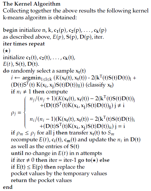
Here the t designates temporary values. The temporary values are finally transferred to the pocket values and thus constitute the output.

In addition the expression behind the brace describes the updates of the centres (means) as obtained in section 11. Using Gallant’s method it is possible to fix a number of repetitions of the algorithm and then select the best one obtained. This is standard practice.

13. Experimental Results Reported

In [1] David Arthur and Sergei Vassilitski report the following.

Experiments:

They implemented and tested their k-means++ algorithm in C++ and compared it to k-means. They tested k = 10, 25, 50 with 20 runs each due to randomized seeding processes.

Data Sets Used:

They used four datasets. The first one was a synthetic data set containing 25 centers selected at random from a fifteen dimensional hypercube. They then added points of a Gaussian distribution of variance 1 around each center thus obtaining a good approximation to the optimal clustering around the original centers. The remaining datasets were chosen from real-world examples off the UC-Irvine Machine Learning Repository.

Results Reported:

They observed that k-means++ consistently outperformed k-means, both by achieving a lower target function value, in some cases by several orders of magnitude, and also by having a faster running time. The 𝐷² seeding (the weighting given in (32)) was slightly slower than uniform seeding, but it still lead to a faster algorithm since it helped the local search converge after fewer iterations. The synthetic ex- ample was a case where standard k-means did very badly. Even though there was an “obvious” clustering, the uniform seeding would inevitably merge some of these clusters, and the local search would never be able to split them apart. The careful seeding method of k-means++ avoided this problem altogether, and it almost always attained the optimal clustering on the synthetic dataset. As far as applications go it should be mentioned that it is possible to exploit this algorithm for maximum likelihood applications, for details see [21], where the clustering algorithm is used to obtain an approximate solution of the maximum likelihood problem for normal mixtures.

The difference between k-means and k-means++ on the real world data sets was also substantial. Without exception k-means++ achieved a significant improvement over k-means. In every case, k-means++ achieved at least a 10% improvement in accuracy over k-means, and it often per- formed much better. Indeed, on the Spam and Intrusion datasets, k-means++ achieved target function values 20 to 1000 times smaller than those achieved by standard k-means. Each trial also completed two to three times faster, and each individual trial was much more likely to achieve a good clustering Of course, these results cannot be directly transferred to the kernel algorithm, since that is dependent on the particular kernel employed. The choice of kernel again depends on the particular problem to be handled. Nevertheless, they provide good indications as to how to improve the classical algorithm in feature space.

14. Conclusion

By adopting the initialization suggested by Arthur and Vassilitski the kernel version of Duda’s algorithm could be improved. In particular it seems that the well-known problems concerning getting stuck in local extrema have been avoided to some extent. This way the special advantages of the iterative algorithm originally described by Duda can be fully exploited. Indeed experimental results presented by Arthur and Vassilitski substantiate that claim. Moreover a trivial modification allows a quantification of improvements obtained after the initialization. Thus an easy application of trial and error methods using a ratchet is obtained. This is similar to a method used in supervised learning (Gallant’s Pocket Algorithm). As far as applications go it should be pointed out that it is possible to exploit this algorithm for maximum likelihood applications, where the clustering al- gorithm is used to obtain an approximate solution of the maximum likelihood problem for normal mixtures. In this context it should also be mentioned that by Arthur and Vassilitski certain generalizations of the k-means++ algo- rithm are considered yielding only slight weaker results. The author also considered Bregman Divergencies and the so-called Jensen Bregman. This can be utilized to obtain a generalization by appealing to the Reproducing Kernel Hilbert Space, see section 3.

The experimental results described above give clear indications towards the advantages of careful seeding. However, further investigations are needed to find suitable kernels for the particular problems considered. Thus there is still room for much future work.

1. B.-J. Falkowski, “Maximum likelihood estimates and a kernel k-means iterative algorithm for normal mixtures”, “USB Proceedings IECON 2020 The 46th Annual Conference of the IEEE Industrial Electronics Society”, Online Singapore, doi:10.1109/IECON43393.2020.9254276.
2. J. Shawe-Taylor, N. Cristianini, Kernel Methods for Pattern Analysis, Cambridge University Press, 2004.
3. B.-J. Falkowski, “On certain generalizations of inner product similar- ity measures”, Journal of the American Society for Information Science, vol. 49, no. 9, 1998.
4. G. Salton, Automatic Text Processing, Addison-Wesley Series in Com- puter Science, 1989.
5. N. Aronszajn, “Theory of reproducing kernels”, AMS, 1950.
6. G. Wahba, “Support vector machines, reproducing kernel hilbert spaces, and randomized gacv”, “Advances in Kernel Methods, Sup- port Vector Learning”, MIT Press, 1999.
7. G. Wahba, “An introduction to reproducing kernel hilbert spaces and why they are so useful”, “IFAC Publications”, Rotterdam, 2003.
8. A. Gretton, “Introduction to rkhs and some simple kernel algorithms”, 2019, uCL.
9. D. Knuth, The Art of Computer Programming. Vol. 1, Fundamental Algo- rithms, 2nd Edition, 1973.
10.  “Polynomial kernel”, https://en.wikipedia.org/wiki/ Polynomial_kernel, accessed: 2024-03-24.
11. I. Schoenberg, “On certain metric spaces arising from euclidean spaces and their embedding in hilbert space”, Annals of Mathematics, vol. 38, no. 4, 1937.
12. I. Schoenberg, “Metric spaces and positive definite functions”, Trans- actions of the American Mathematical Society, vol. 41, 1938.
13. C. Bishop, Neural Networks for Pattern Recognition, Oxford University Press, 2013, reprinted.
14. B.-J. Falkowski, “Mercer kernels and 1-cohomology”, N. Baba, R. Howlett, L. Jain, eds., “Proc. of the 5th Intl. Conference on Knowl- edge Based Intelligent Engineering Systems and Allied Technologies (KES 2001)”, IOS Press, 2001.
15. B.-J. Falkowski, “Mercer kernels and 1-cohomology of certain semi- simple lie groups”, V. Palade, R. Howlett, L. Jain, eds., “Proc. of the 7th Intl. Conference on Knowledge-Based Intelligent Information and Engineering Systems (KES 2003)”, vol. 2773 of LNAI, Springer Verlag, 2003.
16. A. Jain, “Data clustering: 50 years beyond k-means”, Pattern Recogni- tion Letters, 2009, doi:10.1016/j.patrec.2009.09.011.
17. R. Duda, P. Hart, D. Stork, Pattern Classification, Wiley, 2017, reprinted.
18. R. Chitta, “Kernel-clustering based on big data”, Ph.D. thesis, MSU, 2015.
19. “Kernel clustering”, http://www.cse.msu.edu>cse902>ppt>Ker.
    .., last visited: 20.01.2019.
20. B.-J. Falkowski, “A kernel iterative k-means algorithm”, “Advances in Intelligent Systems and Computing 1051, Proceedings of ISAT 2019”, Springer-Verlag, 2019.
21. B.-J. Falkowski, “Bregman divergencies, triangle inequality, and max- imum likelihood estimates for normal mixtures”, “Proceedings of the 2022 Intelligent Systems Conference (Intellisys)”, vol. 1, Springer, 2022, doi:10.1007/978-3-031-16072-1_12.
22. S. Gallant, “Perceptron-based learning algorithms”, IEEE Transactions on Neural Networks, vol. 1, no. 2, 1990.
23. D. Stork, “Solution manual to accompany pattern classification, 2nd ed.”, PDF can be obtained via Wiley.
24. D. Arthur, S. Vassilitski, “k-means++: The advantages of careful seed- ing”, “Proceedings of the Eighteenth Annual ACM-SIAM Symposium on Discrete Algorithms (SODA)”, 2007.
25. S. Har-Peled, B. Sadri, “How fast is the k-means method?”, “ACM- SIAM Symposium on Discrete Mathematics (SODA)”, 2005.
26. “Kernel k-means and spectral clustering”, https://www.cs.utexas. edu/~inderjit/public_papers/kdd_spectral_kernelkmeans. pdf, last visited: 19.06.2018.

Citations by Dimensions

Citations by PlumX

Crossref Citations

This paper is currently not cited.

No. of Downloads per Month

No. of Downloads per Country