Evaluation of Equivalent Aacceleration Factors of Repairable Systems in a Fleet: a Process-Average-Based Approach

(This article belongs to the Special Issue on Special Issue on Multidisciplinary Sciences and Advanced Technology (SI-MSAT 2024) and the Section Operations Research and Management Science (ORM))
Export Citations
Cite
Jiang, R. , Zhang, K. , Xu, X. and Cao, Y. (2024). Evaluation of Equivalent Aacceleration Factors of Repairable Systems in a Fleet: a Process-Average-Based Approach. Journal of Engineering Research and Sciences, 3(10), 44–54. https://doi.org/10.55708/js0310005
Renyan Jiang, Kunpeng Zhang, Xia Xu and Yu Cao. "Evaluation of Equivalent Aacceleration Factors of Repairable Systems in a Fleet: a Process-Average-Based Approach." Journal of Engineering Research and Sciences 3, no. 10 (October 2024): 44–54. https://doi.org/10.55708/js0310005
R. Jiang, K. Zhang, X. Xu and Y. Cao, "Evaluation of Equivalent Aacceleration Factors of Repairable Systems in a Fleet: a Process-Average-Based Approach," Journal of Engineering Research and Sciences, vol. 3, no. 10, pp. 44–54, Oct. 2024, doi: 10.55708/js0310005.
Research on repairable systems in a fleet is mainly concerned with modelling of the failure times using point processes. One important issue is to quantitatively evaluate the heterogeneity among systems, which is usually analyzed using frailty models. Recently, a fleet heterogeneity evaluation method is proposed in the literature. This method describes the heterogeneity with the relative dispersion of equivalent acceleration factors (EAFs) of systems, which is defined as the ratio of the mean times between failures (MTBFs) of a system and a reference system. A main drawback of this method is that the MTBFs of a specific system and the reference system are estimated at different times while the MTBF estimated at different time can be different. This paper aims to address this issue by proposing an improved method. The proposed method uses an “average process” as the reference process and estimates the MTBFs of systems and the reference system at a common time point. This leads to more robust MTBF estimates. Three datasets are analyzed to illustrate the proposed method and its superiority.
1. Introduction
The literature on repairable systems is vast and mainly concerned with modelling of the failure times using point processes [1-2]. The repairable systems that most of the literature deals with can be roughly divided into two categories: (a) multi-component repairable systems composed by non-identical components, and (b) repairable systems in a fleet composed by identical or similar units. In this paper, we focus on the repairable systems in a fleet.
The reliability modeling of repairable systems in a fleet involves a number of issues, including:
- Failure trend analysis [3-4] and failure pattern analysis [5-6]. The former deals with the behavior of the failure occurrence rate or failure intensity, e.g., increasing, decreasing or non-monotonic over time; and the latter aims to identify typical shape types of failure intensity function.
- Fleet heterogeneity evaluation and/or modeling [7-10]. Basic models are frailty models [11-13] and the equivalent acceleration factor model can be viewed as an exception [14].
- Reliability model selection [15-16] and development of models and/or methods for modeling the data with different types of information or covariates (e.g., failure causes and modes) and different types of censoring [17-26].
- Maintenance quality evaluation [27], maintenance decision optimization [14, 23, 28], and prediction of number of failures [29-30].
The focus of this paper is on the evaluation of heterogeneity of repairable systems in a fleet.
Different from the frailty models, Jiang et al. [14] recently propose a heterogeneity evaluation method for repairable systems in a fleet. It estimates the mean time between failures (MTBFs) of individual systems at the right end point of the observation window of each system and defines the equivalent acceleration factor (EAF) of a specific system as the ratio between the MTBFs of this system and a reference system, which is the one whose failure number is the largest among all the systems. The fleet heterogeneity is measured by the ratio of the sample average and standard deviation of EAFs of all the systems. The smaller this ratio is, the greater the heterogeneity of the fleet is. Generally, the observation windows of systems are different so that the MTBFs of different systems are estimated at different time points while the MTBF estimated at different time is different and can be considerably overestimated when the failure number is small. As a result, the EAFs estimated from the above-mentioned heterogeneity evaluation method can be unreliable. This paper aims to address this research gap through proposing an improved method to estimate the EAFs and MTBFs of systems. The proposed method uses an “average system” as the reference system or process, whose mean cumulative function (MCF) equals to the MCF of the fleet. The EAF of a system is estimated as the ratio between the MCFs of the system and fleet (or reference system) at the right end point of the observation window of the system; and the MTBF of the system is estimated as the product of the EAF and fleet MTBF. A unique advantage of using the average process as the reference process is that any data point on the MCF of a specific unit always corresponds to a data point on the MCF of the average process. The reference process defined in [14] does not have such a property. This property makes it possible to assess the MTBFs at the same time. Three datasets are analyzed to illustrate the proposed method and its superiority.
The paper is organized as follows. The proposed method is presented in Section 2, compared with the frailty model in Section 3, and illustrated in Section 4. The paper is concluded in Section 5.
2. Proposed method
2.1. Nelson MCF estimator
Consider a fleet of nominally identical repairable systems, and each system is called a unit. Failure point processes of units are randomly censored on the right. Let 𝑡𝑖𝑗 denote the time to the 𝑗th failure of the 𝑖th unit, and 𝑥𝑖𝑗 = 𝑡𝑖𝑗 − 𝑡𝑖,𝑗 −1 (𝑡𝑖,0 = 0) denote the inter-failure time. The failure point process data are given by
$$\{ t_{ij} \leq \tau_i,\ 1 \leq i \leq n,\ 1 \leq j \leq n_i \} \tag{1}$$
where 𝜏𝑖 is the censored time of the 𝑖th unit, and 𝑛𝑛𝑖𝑖 is the failure number of the 𝑖th unit. The fleet is single censoring if 𝜏1 = 𝜏2 = ⋯= 𝜏𝑛; otherwise, it is multiple censoring. The total failure number of the fleet is \(N = \sum_{i=1}^{n} n_i\), and the censoring time of the fleet is defined as
$$\tau = \max_i (\tau_i).\tag{2}$$
The total time on test (TTT, or 𝑇3 for short) of the fleet at 𝜏 is \(T_3(\tau) = \sum_{i=1}^{n} \tau_i\), and the fleet MTBF evaluated at 𝜏 is estimated as
$$\mu_F = T_3(\tau)/N.\tag{3}$$
A failure point process can be characterized by the MCF of the fleet, which is the mean cumulative number of failures per unit. The MCF can be used to predict the total number or cost of repairs of the fleet in a future period and to determine an optimum retirement age of a system [7]. To estimate the MCF of the fleet, the data given by (1) are sorted in an ascending order. Let 𝑡𝑘 (1 ≤ 𝑘 ≤ 𝑁) denote the 𝑘th smallest value of 𝑡𝑖𝑗 ’s, and 𝑠(𝑡𝑘) denote the number of units at risk at time 𝑡𝑘. For a single censoring fleet, 𝑠(𝑡𝑘) = 𝑛; for a multiple censoring fleet, 𝑠(𝑡𝑘) decreases with 𝑘 and tends to 1. The Nelson MCF estimator is given by [7-8]
$$M_N(t_k) = M_N(t_{k-1}) + \frac{1}{s(t_k)}, \quad t_0 = 0, \, M_N(0) = 0.\tag{4}$$
Equation (4) is a staircase function with \(M_N(t_k^-) = M_N(t_{k-1}^+)\). That is, the MCF at 𝑡𝑘 has two values. To make the MCF at 𝑡𝑘 unique, a smoothed MCF is defined as
$$M(t_k) = \frac{M_N(t_{k-1}) + M_N(t_k)}{2}\tag{5}$$
An MCF-based fleet MTBF can be estimated as
$$\mu_{FN} = \frac{\tau}{M(\tau)}\tag{6}$$
Thus, we have two the MTBF estimates obtained from (3) and (6), respectively. For a single censoring fleet, we have 𝑇3(𝜏)=𝑛𝜏 and 𝑀(𝜏)=𝑁/𝑛. From (6) yields
$$\mu_{FN} = \frac{T_3(\tau)}{\frac{N}{n}} = \frac{T_3(\tau)}{N} = \mu_F\tag{7}$$
In this case, (6) is consistent with (3). For a multiple censoring fleet, the MTBF estimated from (6) is generally different from the MTBF estimated from (3). As mentioned by Nelson [7], the Nelson MCF estimator for large 𝑡 is not robust for a multiple censoring fleet since 𝑠(𝑡) decreases as 𝑡 increases. Therefore, the fleet MTBF estimated by (3) is preferred.
2,2, Robust MCF estimator
To improve the Nelson MCF estimator, a robust estimator is recently proposed by [14]. Specific details are outlined as follows.
Suppose that an ordered dataset (𝑡𝑘, 1 ≤ 𝑘 ≤ 𝑁) is collected from a multiple censoring fleet with 𝑛𝑛 units. An equivalent operating time \(t_k^*\) associated with 𝑡𝑘 is defined by
$$t_k^* = \frac{T_3(t_k)}{n}\tag{8}$$
Define an equivalent single censoring fleet with 𝑛𝑛 units, whose censoring time is defined as
$$\tau^* = \frac{T_3(\tau)}{n}\tag{9}$$
Its MCF is estimated by (4) and (5) with 𝑡𝑘 and 𝑠(𝑡𝑘) being replaced by \(t_k^*\) and 𝑛, respectively. The MCF obtained in such a way is called as the robust MCF estimator. Its robustness results from the fact that the increment of the MCF is 1/𝑛, which is smaller than the MCF increment of the Nelson estimator, 1/𝑠(𝑡𝑘).
Based on the robust MCF, the fleet MTBF can be estimated as
$$\mu_{FJ} = \frac{\tau^*}{M(\tau^*)}\tag{10}$$
It is noted that 𝑀(𝜏∗) = 𝑁/𝑛. Using this relation and (9) to (10) yields
$$\mu_{FJ} = \frac{T_3(\tau)}{N} = \mu_F\tag{11}$$
That is, (11) is consistent with (3) and hence the appropriateness of the robust MCF estimator is confirmed.
2.3. Equivalent acceleration factors
[14] estimate the MTBF of the 𝑖th unit as
$$\mu_i = \frac{\tau_i}{n_i}\tag{12}$$
The unit that has the largest failure number is selected as the reference unit, whose MTBF and censoring time are denoted as 𝜇𝑅 and 𝜏𝑅, respectively. The EAF of the 𝑖th unit is defined as
$$\alpha_i = \frac{\mu_i}{\mu_R}\tag{13}$$
Clearly, 𝛼𝑖 can be viewed as a normalized MTBF, which is dimensionless.
Let 𝜇𝛼 and 𝜎𝛼 denote the mean and standard deviation of all the EAF values, respectively. The fleet heterogeneity is measured by
$$\rho_{\alpha} = \frac{\mu_{\alpha}}{\sigma_{\alpha}}\tag{14}$$
[14] suggest 1.96 as the critical value of 𝜌𝛼. If 𝜌𝛼 > 1.96, the fleet is thought to be homogeneous; otherwise, heterogeneous.
Generally, the MTBF estimated at different time is different and it is negatively correlated with unit age. It is noted that 𝜇𝑖 is estimated at 𝜏𝑖 ≤ 𝜏 and 𝜇𝑅 is estimated at 𝜏𝑅, which is generally different from 𝜏𝑖. That is, 𝜇𝑖 and 𝜇𝑅 is estimated at different time points. When 𝜏𝑖 and 𝜏𝑅 are significantly different, the EAF estimated by (13) is unreliable. To improve, 𝜇𝑖 and 𝜇𝑅 should be estimated at the same time point 𝜏𝑖. In this case, (13) is revised as
$$\alpha_i = \frac{\mu_i}{\mu_R(\tau_i)}\tag{15}$$
where 𝜇𝑅(𝜏𝑖) is the MTBF of the reference unit estimated at 𝜏𝑖 by interpolation or extrapolation. To facilitate the evaluation of 𝜇𝑅(𝜏𝑖) and obtain a more robust estimate of 𝜇𝑅(𝜏𝑖), it is necessary to redefine the reference unit. This will yield an improved EAF evaluation method.
2.4. Improved EAF evaluation method
We define a virtual unit as the reference unit, its failure process equals to the “average process” of the fleet, and its MCF is given by the Nelson estimator of the fleet MCF. In this case, we have
$$\mu_R(\tau_i) = \frac{\tau_i}{M(\tau_i)}, \quad \mu_i = \frac{\tau_i}{M_i(\tau_i)}\tag{16}$$
where 𝑀𝑖(.) is the MCF of the 𝑖th unit. If 𝜏𝑖 > 𝑡𝑛𝑖, 𝑀𝑖(𝜏𝑖) = 𝑛𝑖; if 𝜏𝑖 = 𝑡𝑛𝑖, 𝑀𝑖(𝜏𝑖) = 𝑛𝑖 − 0.5. Using (16) to (15) yields
$$\alpha_i = \frac{M(\tau_i)}{M_i(\tau_i)}\tag{17}$$
Assume that the EAF estimated from (17) is approximately a constant. That is, 𝛼𝑖(𝜏𝑖) ≈ 𝛼𝑖(𝜏). Under this assumption, the MTBFs of the units evaluated at 𝜏𝜏 can be estimated as
$$\mu_i = \alpha_i \mu_F\tag{18}$$
where 𝜇𝐹 is given by (3). Thus, the MTBFs of all the units are evaluated at a common time 𝜏.
It is noted that (18) is the MTBF of the 𝑖th unit evaluated at 𝜏𝜏 while (12) is the MTBF of the 𝑖th unit evaluated at 𝜏𝑖. The two estimates are usually different and their relative error is given by
$$\varepsilon_i = \left| 1 – \frac{\mu_i(\tau_i)}{\mu_i(\tau)} \right|\tag{19}$$
When 𝜏𝑖 is much smaller than 𝜏, 𝜀𝑖 may be large, as to be illustrated by Figures 1 and 3 in Section 4.
3. Comparison of the EAF-based approach with frailty model
Traditionally, the heterogeneity of repairable systems in a fleet is modeled by a frailty model [11-13, 31]. In this section, we compare the EAF-based approach with the frailty model and illustrate the conclusions obtained from comparison analysis using a real-world example.
3.1. Frailty model
Consider the failure point processes given by (1). In the context of frailty analysis, each system in the fleet has its own failure intensity; and the effect of the heterogeneity on the failure process of a system is described a non-negative random variable called the frailty. The frailty model is defined in terms of the intensity function of a failure process, given by
$$m(t|Z) = Z m_0(t)\tag{20}$$
where 𝑚0(𝑡) is the baseline failure intensity function. Equation (20) is actually a proportional intensity model [32]. According to (20), the intensity function of the 𝑖th unit can be written as
$$m_i(t) = z_i m_0(t)\tag{21}$$
where 𝑧𝑖 is the frailty of the 𝑖th unit.
To specify a frailty model, one needs to specify the type of the repair process (i.e., minimal, imperfect or perfect repair) and the distribution of the frailty. For a minimal repair process, the non-homogeneous Poisson process with a power-law MCF is assumed. The power-law MCF is given by
$$M(t) = \left( \frac{t}{\eta} \right)^{\beta}\tag{22}$$
The frailty is usually assumed to follow the gamma distribution with scale parameter 𝜃 and shape parameter 1/𝜃. The expectation of this distribution is one and the variance is 𝜃. A large value of 𝜃 indicates that there exists heterogeneity between the systems. This frailty model has three parameters (i.e., 𝛽,𝜂; 𝜃) to be estimated. For the data given by (1), the parameters can be estimated using the maximum likelihood estimation method. Since 𝑧𝑖 is unobserved, the ordinary likelihood function has to be replaced by the marginal likelihood obtained by unconditioning with respect to 𝑧𝑖.
Once the parameters are specified, the frailty 𝑧𝑖 of the 𝑖th unit can be estimated. For the above-mentioned frailty model, the frailty of the 𝑖th unit is estimated by
$$z_i = \left( \frac{1}{\theta} + n_i \right) \Big/ \left[ \frac{1}{\theta} + M(\tau_i) \right]\tag{23}$$
3.2. Comparison of the EAF-based approach with the frailty model
We compare the EAF-based approach with the frailty model from four aspects: definitions of EAF and frailty, evaluation methods of heterogeneity, determination of fleet heterogeneity and interpretations of EAF and frailty.
Definition of EAF and frailty: Both the EAF and frailty are defined relative to an “average” system; the EAF is defined in terms of the MTBF, and the frailty is defined in terms of intensity function. From (23), the frailty is asymptotically reciprocally proportional to the EAF as 𝜃 → ∞ . These imply that the two models are somehow similar and closely related.
Evaluation of heterogeneity: Parameter of the frailty model describes the heterogeneity and is estimated using a parametric approach. The approach needs to make the assumptions about the types of repair process and frailty distribution, and the parameter estimation needs to use an unconditional approach. These make this approach complex and the results unreliable due to possible misspecification. On the other hand, the EAF-based approach does not make any assumptions since it is essentially a non-parametric approach. Therefore, it is simpler and more reliable than the frailty model.
Determination of fleet heterogeneity: The EAF-based approach defines a critical value of to objectively determine whether the heterogeneity exists while the frailty-based approach does not define such a critical value so that the determination of fleet heterogeneity is subjective to some extent.
Interpretation of EAF and frailty: The EAF of a system is the ratio of two statistics (i.e., system MTBF and fleet MTBF) while the frailty is the ratio of two functions (i.e., system intensity and baseline intensity). Thus, the former can be viewed as being “observable” since the MTBF can be directly computed from the data while the latter is unobserved since it can be only estimated based on the data and assumed models.
3.3. A robust estimate for frailty of a system
It is noted that the frailty given by (23) is highly sensitive to the value of 𝜃: when 𝜃 → 0, 𝑧𝑖 →1; and when \(\theta \to \infty, \; z_i \to \frac{n_i}{M(\tau)} = \frac{1}{\alpha_i}\). To make 𝑧𝑖 robust, we define a non-parametric estimate of the frailty. Consider the single censoring case with 𝜏𝑖 = 𝜏,(1 ≤ 𝑖 ≤ 𝑛). Integrating the two sides of (21) from zero to 𝜏, we have
$$\textit{LHS} = n_i,\; \textit{RHS} = z_i M(\tau)\tag{24}$$
Letting LHS = RHS yields
$$z_i = \frac{n_i}{M(\tau)} = \frac{1}{\alpha_i}\tag{25}$$
This estimate is independent of 𝜃 and can be interpreted as the ratio of the system’s failure numbers and expected failure number of the fleet in a common observation window (0,𝜏). The frailty given by (25) is reciprocally proportional to the EAF. According to this definition, the frailty becomes “observable”. The definition can be extended to the multiple censoring case: the frailty of system 𝑖 is the ratio of the system’s failure numbers and expected failure number of the fleet evaluated at 𝜏𝑖.
3.4. Example 1
In this subsection, we illustrate the frailty-based and EAF-based approaches by a real-world example.
3.4.1. Data
The example comes from [31] and deals with the failure processes of 9 sugarcane harvesters, observed in a common period of 200 days. [31] Present the failure time data of the systems with a figure, from which we extract the data shown in the first two rows of Table 1.
Table 1: Failure numbers of sugarcane harvesters in 200 days
| 𝑖 | 1 | 2 | 3 | 4 | 5 | 6 | 7 | 8 | 9 | |
| 𝑛𝑖 | 11 | 14 | 14 | 15 | 19 | 14 | 11 | 13 | 16 | 0.1752 |
𝑧𝑖 , (23) | 0.9989 | 0.9991 | 0.9991 | 0.9991 | 0.9994 | 0.9991 | 0.9989 | 0.9990 | 0.9992 | 0.0002 |
𝑧𝑖 , (25) | 0.7795 | 0.9921 | 0.9921 | 1.063 | 1.346 | 0.9921 | 0.7795 | 0.9213 | 1.134 | 0.1799 |
| 𝜇𝑖 | 18.18 | 14.29 | 14.29 | 13.33 | 10.53 | 14.29 | 18.18 | 15.38 | 12.5 | 0.1704 |
| 𝛼𝑖 | 1.283 | 1.008 | 1.008 | 0.941 | 0.743 | 1.008 | 1.283 | 1.085 | 0.882 | 0.1704 |
3.4.2. Results of the frailty-based approach
In [31], the authors estimated assume that the repair is perfect, the time to failure follows the Weibull distribution with shape parameter 𝛽 and scale parameter 𝜂, and the frailty follows the gamma distribution with parameter 𝜃. The maximum likelihood estimates (MLEs) of the parameters are (𝛽,𝜂; 𝜃)= (1.32, 15.02; 0.56×10⁻⁴). Since the estimate of 𝜃 is nearly equal to zero, the unobserved heterogeneity among the systems is deemed to be non-existent. The frailties estimated from (23) are shown in the third row of Table 1 and the frailties estimated from (25) are shown in the fourth row. The last column shows the coefficient of variation (𝛿) of the nine values of each row. It is expected that 𝛿(𝑧𝑖) should be close to 𝛿(𝑛𝑖). However, (23) does not meet this expectation while (25) meets the expectation, and hence its appropriateness is confirmed.
3.4.3. Results of the proposed approach
Since the observation windows of the systems are the same, it is easy to evaluate the MCF and MTBF of the fleet, which are 𝑀(200) = 14.11 and 𝜇𝐹 = 14.17 days, respectively. It is also easy to calculate the MTBFs and EAFs of individual systems using the following relations
$$\mu_i = 200/n_i,\; \alpha_i = M(200)/n_i\tag{26}$$
The results are shown in the last two rows of Table 1. The average and standard deviation of the EAFs are 𝜇𝛼 = 1.0267 and 𝜎𝛼 = 0.1749, respectively; and their ratio is 𝜌𝛼 = 5.870, which is much larger than 1.96. Therefore, the fleet is homogeneous. This conclusion is consistent with the one of [31] though 𝛿(𝑧𝑖) obtained from (23) is significantly different from 𝛿(𝑧𝑖) obtained from (25).
4. Further illustrations
In this section, we further illustrate the proposed approach and its superiority using two examples, which have been analyzed by [14].
4.1. Example 2
4.1.1. Data
Consider a fleet of 10 units, and each has a power-law MCF given by (22) with parameters 𝛽 = 1.5 and 𝜂 = 100. A failure is restored by minimal repair; and the censoring time of each unit is randomly generated from the uniform distribution over (0, 500) so that 𝜏 𝜏𝑖 >𝑡𝑛𝑖. The randomly generated data are shown in the upper part of Table 2 and the censoring times of units are shown in the last row. From the table yields four important statistics:
$$N = 46, \; \tau = 470.9, \; T_3(\tau) = 2601.7, \; \mu_F = 56.56.\tag{27}$$
Table 2: Failure processes of units
Unit | 1 | 2 | 3 | 4 | 5 | 6 | 7 | 8 | 9 | 10 |
| 𝑡1 | 245 | 131 | 17 | 105 | 19 | 70 | 108 | 32 | ||
| 𝑡2 | 293 | 194 | 51 | 209 | 49 | 174 | 188 | 103 | ||
| 𝑡3 | 353 | 277 | 56 | 235 | 195 | 235 | ||||
| 𝑡4 | 356 | 278 | 188 | 255 | 215 | |||||
| 𝑡5 | 378 | 279 | 206 | 262 | 271 | |||||
| 𝑡6 | 401 | 324 | 216 | 270 | 356 | |||||
| 𝑡7 | 424 | 231 | 281 | |||||||
| 𝑡8 | 466 | 249 | 331 | |||||||
| 𝑡9 | 251 | |||||||||
| 𝑡10 | 338 | |||||||||
| 𝑡11 | 372 | |||||||||
𝑡i | 470.9 | 336.1 | 50.5 | 441.3 | 348.3 | 111.6 | 92.8 | 374.5 | 239.4 | 136.3 |
4.1.2. Evaluation of MTBF and EAF
The information that the approach of in [14], the authors estimated requires for estimating the MTBFs and EAFs of units are shown in the first three columns of Table 3; and the estimated MTBFs and EAFs are shown in the 4th and 5th columns. As can be seen, using the approach of [14] cannot estimate the MTBFs and EAFs of Units 3 and 6 due to 𝑛3 = 𝑛6 = 0.
Although no failure occurs for Units 3 and 6, these two units can and should be included in the computation of MCF since their censoring information has an influence on 𝑠(𝑡𝑘). The results obtained from the proposed approach are shown in the 6th to 8th columns. Different from the approach of [14], which first estimates 𝜇𝑖 (at 𝜏𝑖) and then estimates 𝛼𝑖, the improved method first estimates 𝛼𝑖 (at 𝜏𝑖) and then estimates 𝜇𝑖 (at 𝜏).
Table 3: MTBFs and EAFs of units obtained from two methods
Unit | Jiang et al. [14] | Improved approach | ||||||
| 𝜏𝑖 | 𝑛𝑖 | 𝜇𝑖 (12) | 𝛼𝑖 | 𝑀(𝜏𝑖) | 𝛼𝑖 (17) | 𝜇𝑖 (18) | ||
1 | 470.9 | 8 | 58.86 | 1.467 | 10.13 | 1.267 | 71.65 | 0.1785 |
2 | 336.1 | 6 | 56.02 | 1.396 | 6.051 | 1.009 | 57.04 | 0.0180 |
3 | 50.50 | 0 | 0.4000 | (0.7315) | (41.37) | |||
4 | 441.3 | 11 | 40.12 | 1.000 | 9.135 | 0.8304 | 46.97 | 0.1458 |
5 | 348.3 | 8 | 43.54 | 1.085 | 6.301 | 0.7876 | 44.55 | 0.0227 |
6 | 111.6 | 0 | 1.108 | (2.027) | (114.6) | |||
7 | 92.80 | 2 | 46.40 | 1.157 | 0.7333 | 0.3667 | 20.74 | 1.237 |
8 | 374.5 | 6 | 62.42 | 1.556 | 7.635 | 1.272 | 71.97 | 0.1327 |
9 | 239.4 | 3 | 79.80 | 1.989 | 3.251 | 1.084 | 61.29 | 0.3019 |
10 | 136.3 | 2 | 68.15 | 1.699 | 1.251 | 0.6256 | 35.38 | 0.9261 |
Since the reference process is an “average process”, it is possible to estimate the MTBFs and EAFs of Units 3 and 6 based on the following two assumptions:
(a) The average of EAFs of all the units equals to 1, and
(b) From (17) we can assume that 𝛼𝑖 = 𝑐M(𝜏𝑖) for 𝑖 = 3 and 6.
The value of 𝑐 can be estimated from the first assumption, which is 1.829. From the second assumption yields 𝛼3 = 0.7315 and 𝛼6 = 2.027. Further, from (18) yields 𝜇3 = 41.37 and 𝜇6 = 114.6. These estimates are bracketed in Table 3.
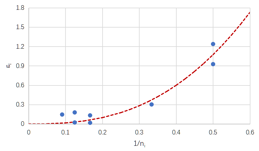
The last column shows the relative errors between the MTBFs estimated from (12) and (18). To examine the influence of censoring time 𝜏𝑖 (or failure number 𝑛𝑖) on the accuracy of MTBF estimate, we examine the plot of 𝜀𝑖 vs. 𝑛𝑖 shown in Figure 1. As seen from the figure, 𝜀𝑖 quickly increases as 𝑛𝑛𝑖𝑖 decreases (or 1/𝑛𝑖 increases), implying that the MTBF estimates obtained from (12) and (18) are nearly the same when 𝑛𝑖 is large. Since the estimate obtained from (12) is accurate when 𝑛𝑖 is large, this actually validates the appropriateness of (18).
4.1.3. Estimates of fleet MTBF
As mentioned in Section 2, the fleet MTBF can be estimated by a TTT-based approach given by (3) and by an MCF-based approach given by (6). We illustrate that they are different for multiple censoring case.
From (27) and Table 3 we have 𝜏 = 𝜏1 = 470.9 and 𝑀(𝜏) = 𝑀(𝜏1)=10.13. Applying these to (6) yields 𝜇FN = 46.46. On the other hand, from (3) we have 𝜇FN = 56.56. This implies that the MCF-based approach underestimates the fleet MTBF with a relative error of 17.85%. This also indirectly illustrates that the Nelson MCF estimator can be inaccurate for the multiple censoring case, and its accuracy can be measured by the relative error given by
$$\varepsilon_F = \left| 1 – \frac{\mu_{FN}}{\mu_F} \right|.
\tag{28}$$
The larger the relative error is, the less accurate the Nelson MCF estimator is.
4.1.4. Heterogeneity evaluation
The computational results of the heterogeneity are shown in Table 4. The results obtained from the approach of [14] are shown in the second row, the results obtained from the improved method with the EAFs of Units 3 and 6 being excluded are shown in the third row, and the results obtained from the improved method with the EAFs of Units 3 and 6 being included are shown in the last row. As seen, the values of 𝜌𝛼 for these three cases are quite different, but they all are larger than 1.96, implying that the fleet is homogeneous.
Table 4: Fleet heterogeneity measures obtained from different methods
Approach | Units 3 and 6 | 𝜇𝛼 | 𝜎𝛼 | 𝜌𝛼 |
[14] | Excluded | 1.419 | 0.3340 | 4.248 |
This paper | Excluded | 0.9052 | 0.3153 | 2.871 |
Included | 1.000 | 0.4587 | 2.180 |
The difference in 𝜌𝛼 can be explained by a large 𝜀𝐹. Since Units 7, 9 and 10 only have 2, 3 and 2 failures, respectively, their MTBFs are considerably overestimated by (12). This reduces the dispersion of the MTBFs and EAFs and leads to a large value of 𝜌𝛼. This confirms the fact that the units’ EAF estimates obtained from the proposed approach are more robust than those obtained from the approach of [14].
4.1.5. Distribution of EAF
The frailty is usually assumed to follow the gamma distribution with mean one. It is possible to check whether this assumption holds for the EAF. Fitting the EAFs shown in the 7th column of Table 3 to four typical 2-parameter distributions: gamma distribution with parameters 𝑢𝑢 and 𝑣𝑣, Weibull distribution with parameters 𝛽 and 𝜂, normal distribution with parameters 𝜇 and 𝜎𝜎, and lognormal distribution with parameters 𝜇𝑙 and 𝜎𝑙. The MLEs of the parameters are shown in Table 5, where 𝜃1 = 𝑢, 𝛽, 𝜇 or 𝜇𝑙; 𝜃2 = ,𝜂, 𝜎, 𝑣 or 𝜎𝑙; and ln (𝐿) is the log-likelihood value. As seen, the gamma distribution provides the best fit in terms of ln (𝐿).
Table 5: MLEs of distributional parameters
Example 2 | Example 3 | |||||||
| Gamma | Weibull | Normal | Lognormal | Gamma | Weibull | Normal | Lognormal |
| 𝜃1 | 5.498 | 2.434 | 1.000 | -0.0936 | 4.463 | 2.005 | 1.229 | 0.0896 |
| 𝜃2 | 0.1819 | 1.130 | 0.4352 | 0.4413 | 0.2753 | 1.397 | 0.6631 | 0.4580 |
| 𝑙n (𝐿) | -5.034 | -5.423 | -5.871 | -5.074 | -10.37 | -11.50 | -13.11 | -9.459 |
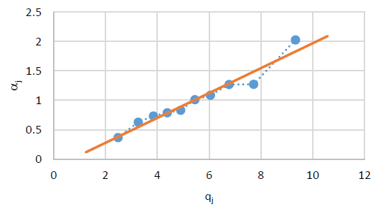
The probability plot of a distribution is often used to check the appropriateness of the distribution. Let 𝛼𝑗 (1 ≤ 𝑗 ≤ 𝑛) denote the ordered EAFs sorted in ascending order, 𝑝𝑗 =(𝑗 − 0.3)/(𝑛 + 0.4), and 𝑞𝑗 = 𝐹−1(𝑝𝑗 ; 𝑢,1) denote the inverse function of the gamma distribution with parameters 𝑢 and 1. The gamma probability plot is given by
$$\alpha_j = v q_j.\tag{29}$$
Figure 2 shows the plot of 𝛼𝑗 vs. 𝑞𝑗 for 𝑢 = 5.498. Regression yields 𝑣 = 0.1879, which is close to the MLE of 𝑣𝑣 with a relative error of 3.29%. This confirms the appropriateness of the gamma distribution for fitting the EAF data.
4.2. Example 3
4.2.1. Data
The data shown in Table 6 come from Proschan [33] and deal with the inter-failure times (in days) of 13 air conditioning systems before overhauls. For this example, the censoring time meets the relation of 𝜏𝑖 = 𝑡𝑛𝑖. From the table, we have
$$N = 192, \; \tau = 2074, \; T_3(\tau) = 18088, \; \mu_F = 94.21.\tag{30}$$
Table 6: Inter-failure times of air conditioning systems
| 𝑗\𝑖 | 1 | 2 | 3 | 4 | 5 | 6 | 7 | 8 | 9 | 10 | 11 | 12 | 13 |
1 | 194 | 413 | 90 | 74 | 55 | 23 | 97 | 50 | 359 | 50 | 130 | 487 | 102 |
2 | 15 | 14 | 10 | 57 | 320 | 261 | 51 | 44 | 9 | 254 | 493 | 18 | 209 |
3 | 41 | 58 | 60 | 48 | 56 | 87 | 11 | 102 | 12 | 5 | 100 | 14 | |
4 | 29 | 37 | 186 | 29 | 104 | 7 | 4 | 72 | 270 | 283 | 7 | 57 | |
5 | 33 | 100 | 61 | 502 | 220 | 120 | 141 | 22 | 603 | 35 | 98 | 54 | |
6 | 181 | 65 | 49 | 12 | 239 | 14 | 18 | 39 | 3 | 12 | 5 | 32 | |
7 | 9 | 14 | 70 | 47 | 62 | 142 | 3 | 104 | 85 | 67 | |||
8 | 169 | 24 | 21 | 246 | 47 | 68 | 15 | 2 | 91 | 59 | |||
9 | 447 | 56 | 29 | 176 | 225 | 77 | 197 | 438 | 43 | 134 | |||
10 | 184 | 20 | 386 | 182 | 71 | 80 | 188 | 230 | 152 | ||||
11 | 36 | 79 | 59 | 33 | 246 | 1 | 79 | 3 | 2 | ||||
12 | 201 | 84 | 27 | 21 | 16 | 88 | 130 | 14 | |||||
13 | 118 | 44 | 42 | 106 | 46 | 230 | |||||||
14 | 59 | 20 | 206 | 5 | 66 | ||||||||
15 | 29 | 5 | 82 | 5 | 61 | ||||||||
16 | 118 | 12 | 54 | 36 | 34 | ||||||||
17 | 25 | 120 | 31 | 22 | |||||||||
18 | 156 | 11 | 216 | 139 | |||||||||
19 | 310 | 3 | 46 | 210 | |||||||||
20 | 76 | 14 | 111 | 97 | |||||||||
21 | 26 | 71 | 39 | 30 | |||||||||
22 | 44 | 11 | 63 | 23 | |||||||||
23 | 23 | 14 | 18 | 13 | |||||||||
24 | 62 | 11 | 191 | 14 | |||||||||
25 | 16 | 18 | |||||||||||
26 | 90 | 163 | |||||||||||
27 | 1 | 24 | |||||||||||
28 | 16 | ||||||||||||
29 | 52 | ||||||||||||
30 | 95 |
4.2.2. Estimation of MTBF and EAF
The results obtained from the approach of [14] are outlined in the 2nd to the 5th column of Table 7. The Nelson MCF estimators at unit censoring times are shown in the 6th column and the EAFs and MTBFs of units obtained from the improved methods are shown in the 7th and 8th columns, respectively. It is noted that 𝜏 = 𝜏7 = 2074 and 𝑀(𝜏) = 𝑀(𝜏7) = 23.74. Applying these to (6) yields 𝜇FN = 87.38, which is slightly smaller than the fleet MTBF shown in (30) with a relative error of 7.25%. An underestimate of 𝜇FN implies an overestimate of 𝑀(𝜏). Compared with Example 2, 𝜀𝐹 is relatively small.
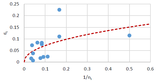
Figure 3 shows the plot of 𝜀𝑖 vs. 𝑛𝑖. As expected, 𝜀𝑖 increases as 𝑛𝑖 decreases. The average and maximum of 𝜀𝑖’s are 0.0683 and 0.2258, respectively, implying that the MTBF estimates obtained from (12) and (18) are fairly close to each other for the current example.
Table 7: MTBFs and EAFs of units obtained from two methods for Example 3
Unit | [14] | Improved approach | 𝜀𝑖 | |||||
| 𝜏𝑖 | 𝑛𝑖 | 𝜇𝑖 (12) | 𝛼𝑖 | 𝑀(𝜏𝑖) | 𝛼𝑖 (17) | 𝜇𝑖(18) |
| |
1 | 493 | 6 | 82.16 | 1.378 | 4.269 | 0.7115 | 67.03 | 0.2258 |
2 | 1851 | 13 | 142.4 | 2.389 | 19.99 | 1.537 | 144.8 | 0.0167 |
3 | 1705 | 24 | 71.04 | 1.191 | 18.80 | 0.7835 | 73.81 | 0.0375 |
4 | 1314 | 12 | 109.5 | 1.837 | 12.95 | 1.080 | 101.7 | 0.0767 |
5 | 1678 | 11 | 152.5 | 2.559 | 18.22 | 1.656 | 156.0 | 0.0221 |
6 | 1788 | 30 | 59.60 | 1.000 | 19.28 | 0.6426 | 60.54 | 0.0155 |
7 | 2074 | 27 | 76.81 | 1.288 | 23.74 | 0.8791 | 82.82 | 0.0725 |
8 | 1539 | 24 | 64.12 | 1.075 | 16.23 | 0.6763 | 63.71 | 0.0065 |
9 | 1800 | 9 | 200.0 | 3.355 | 19.57 | 2.174 | 204.8 | 0.0234 |
10 | 639 | 6 | 106.5 | 1.786 | 6.111 | 1.018 | 95.95 | 0.1100 |
11 | 623 | 2 | 311.5 | 5.226 | 5.933 | 2.966 | 279.5 | 0.1145 |
12 | 1297 | 12 | 108.1 | 1.813 | 12.71 | 1.059 | 99.80 | 0.0830 |
13 | 1287 | 16 | 80.43 | 1.349 | 12.61 | 0.7879 | 74.23 | 0.0836 |
4.2.3. Heterogeneity evaluation
The fleet heterogeneity measure obtained from [14] is 𝜌𝛼 = 1.715, implying that the fleet is heterogeneous. The value of 𝜌𝛼 obtained from the improved method is 1.780, which is very close to the above estimate. The similarity of the results obtained from the two approaches can be explained by the average failure number of units (i.e., 𝑁/𝑛), which is 14.8. For a dataset with a large value of 𝑁/𝑛, both the method of [14] and the improved method will give similar results and draw similar conclusions; otherwise, the results and conclusions are probably different.
4.2.4. Distribution of EAF
Fitting the EAFs shown in the 7th column of Table 7 to the four 2-parameter distributions yields the MLEs of the parameters shown in the RHS of Table 5. In terms of the log-likelihood value, the lognormal distribution provides the best fit to the data. To further validate, we examine the lognormal probability plot. Let 𝑞𝑗 = 𝐹−1(𝑝𝑗 ; 0,1) denote the inverse function of the standard normal distribution. The lognormal probability plot is given by
$$q_j = \frac{\ln(\alpha_j) – \mu_l}{\sigma_l}.\tag{31}$$
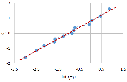
Figure 4 shows the plot of 𝑞𝑗 vs. 𝑙 (𝛼𝑗 ). As can be seen, the plot is concave, implying that the 2-parameter lognormal distribution is not appropriate for fitting the EAF data.
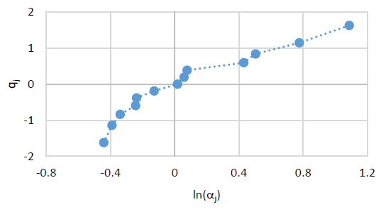
Figure 4 indicates that urther analysis shows that the 3-parameter lognormal distribution with a location parameter 𝛾 can be appropriate for fitting the data. This is validated by the probability plot of the 3-parameter lognormal distribution shown in Figure 5. The least square estimates of the parameters are 𝛾 = 0.5934, 𝜇𝑙 = −1.016, 𝜎𝑙 = 1.259, and the corresponding log-likelihood value is ln(𝐿) = −6.854, which is much larger than the log-likelihood value of the 2-parameter lognormal distribution. From the fitted model yields 𝜌𝛼 = 0.8843, and hence the heterogeneity of the fleet is confirmed.
5. Conclusions
In this paper, we have identified the problems of the heterogeneity evaluation method presented in [14] and proposed an improved method, whose main advantages are:
- it estimates the MTBFs of units at a common time point so that the results are much more reliable than those obtained from the method given in [14], and
- the MTBFs of zero-failure units can be inferred under two reasonable assumptions. This is different from those approaches that exclude the units with an inadequate amount of failure data from the analysis [16].
These have been illustrated by three examples.
The main conclusions and/or findings of the paper have been:
- The MTBFs and EAFs of units estimated from the method [14] and the improved method are fairly consistent if the average failure number of units is large and can be considerably different otherwise.
- The fleet MTBF estimates obtained from the Nelson MCF estimator and TTT approach are different for multiple censoring data.
- The frailty of a system can be defined as the ratio of the system’s failure numbers and expected failure number of the fleet evaluated in a common observation window. Such defined frailty is reciprocally proportional to the EAF.
- A simple distribution such as the 2-parameter gamma or lognormal distribution may be inappropriate for describing the EAF or frailty in the presence of heterogeneity.
In this paper, we have confined to the fleet composed by similar repairable systems rather than multi-component repairable systems and stressed MTBFs of units rather than their trends. The MTBF estimates of the units are based on the constant EAF assumption, whose reasonability requires further validation. The data considered in this paper only contain failure time information without other information such as failure causes, failure modes, maintenance types and censoring types. Analysis for the failure process with such information is a challenging issue and needs further research. Finally, a topic for future study is to develop a cluster analysis method for classifying the units of a heterogeneous fleet (e.g., automated guided vehicles [34]) into several homogeneous groups based on the EAFs of the units.
Conflict of Interest
The authors declare no conflict of interest.
Acknowledgment
The authors would like to thank the referees for their helpful comments and suggestions which have greatly enhanced the clarity of the paper. This work was supported by the ‘Pioneer and Leading Goose + X’ R&D Program of Zhejiang Province, China (2024SJCZX0037) and Wenzhou Major Science and Technology Innovation Projects (ZG2023019).
- Ascher H, Feingold H. Repairable Systems – Modeling, Inference, Misconceptions and their Causes. Marcel Dekker, New York, 1984.
- Lindqvist BH. “Maintenance of repairable systems,” in Complex system maintenance handbook, pp. 235-261, 2008, doi: 10.1007/978-1-84800-011-7_10
- Lindqvist BH. “On the statistical modeling and analysis of repairable systems,” Statistical Science, vol. 21, no. 4, pp. 532-551, 2007, doi: 10.1214/088342306000000448.
- Krivtsov VV. “Practical extensions to NHPP application in repairable system reliability analysis,” Reliability Engineering and System Safety, vol. 92, no. 5, pp. 560-562, 2007, doi: 10.1016/j.ress. 2006.05.002.
- Jiang R, Huang C. “Failure patterns of repairable systems and a flexible intensity function model,” International Journal of Reliability and Applications, vol. 13, no. 2, pp. 81-90, 2012, doi: koreascience.kr/article/JAKO201217752421606.
- R. Jiang, Y. Guo. and strong, “Estimating Failure Intensity of a Repairable System to decide on its Preventive Maintenance or Retirement,” International journal of performability engineering, vol. 10, no. 6, pp. 577-588, 2014, doi: 10.23940/ijpe.14.6.p577.mag.
- Nelson W. “Graphical analysis of system repair data,” Journal of Quality Technology, vol. 20, pp. 24-35, 1988, doi: 10.1080/ 00224065.1988.11979080.
- Nelson W. Recurrent Events Data Analysis for Product Repairs, Disease Recurrences, and Other Applications, Society for Industrial and Applied Mathematics (SIAM): Philadelphia, 2003.
- Asfaw ZG, Lindqvist BH. “Unobserved heterogeneity in the power law nonhomogeneous Poisson process,” Reliability Engineering and System Safety, vol. 134, pp. 59-65, 2015, doi: 10.1016/j.ress.2014.10.005
- Cui D., Sun Q., Xie M., “Robust statistical modeling of heterogeneity for repairable systems using multivariate gaussian convolution processes,” IEEE Transactions on Reliability, vol. 72, no. 4, pp. 1493-1506, 2023, doi: 10.1109/TR.2023.3235889.
- Liu X., Vatn J., Dijoux Y., Toftaker H., “Unobserved heterogeneity in stable imperfect repair models,” Reliability Engineering and System Safety, vol. 203, pp. 107039, 2020, doi: 10.1016/j.ress.2020. 107039.
- Zaki R, Barabadi A, Barabady J, Qarahasanlou AN. “Observed and unobserved heterogeneity in failure data analysis,” Proceedings of the Institution of Mechanical Engineers, Part O: Journal of Risk and Reliability, vol. 236, no. 1, pp. 194-207, 2022, doi: 10.1177/1748006X211022538
- Brown B., Liu B., McIntyre S., Revie M., “Reliability evaluation of repairable systems considering component heterogeneity using frailty model,” Proceedings of the Institution of Mechanical Engineers, Part O: Journal of Risk and Reliability, SAGE journal, vol. 237, no. 4, pp. 654-670, 2023, doi: 10.1177/1748006X221109341.
- Jiang R., Li F., Xue W., Cao Y., et al., “A robust mean cumulative function estimator and its application to overhaul time optimization for a fleet of heterogeneous repairable systems,” Reliability Engineering and System Safety, vol. 236, pp. 109265, 2023, doi: 10.1016/j.ress.2023.109265.
- Garmabaki, AHS, Ahmadi A, Block J, Pham H, Kumar U. “A reliability decision framework for multiple repairable units,” Reliability Engineering & System Safety, vol. 150, pp. 78-88, 2016, http://dx.doi.org/10.1016/j.ress.2016.01.020
- Garmabaki AHS, Ahmadi A, Mahmood YA, Barabadi A. “Reliability modelling of multiple repairable units,” Quality and Reliability Engineering International, vol. 32, no. 7, pp. 2329-2343, 2016, doi: 10.1002/qre.1938
- Weckman GR, Shell RL, Marvel JL. “Modeling the reliability of repairable systems in the aviation industry,” Computers and Industrial Engineering, vol. 40, pp. 51-63, 2001, doi: 10.1016/S0360-8352(00)00063-2.
- Giorgio M, Guida M, Pulcini G. “Repairable system analysis in presence of covariates and random effects,” Reliability Engineering and System Safety, vol. 131, pp. 271-281, 2014, doi: 10.1016/j.ress.2014.04.009.
- Meeker WQ, Hong Y. “Reliability meets big data: opportunities and challenges,” Quality Engineering, vol. 26, pp. 102-116, 2014, doi: 10.1080/08982112.2014.846119.
- Navas MA, Sancho C., Carpio J. “Reliability analysis in railway repairable systems,” International Journal of Quality & Reliability Management, vol. 34, no. 8, pp. 1373-1398, 2017, doi: 10.1108/IJQRM-06-2016-0087.
- Hong Y, Zhang M, Meeker WQ. “Big data and reliability applications: the complexity dimension,” Journal of Quality Technology, vol. 50, no. 2, pp. 135-149, 2018, doi: 10.1080/00224065.2018.1438007.
- Peng W, Shen L, Shen Y, Sun Q, “Reliability analysis of repairable systems with recurrent misuse-induced failures and normal-operation failures,” Reliability Engineering and System Safety, vol. 171, pp. 87-98, 2018, doi: 10.1016/j.ress.2017.11.016.
- Si W, Love E, Yang Q. “Two-state optimal maintenance planning of repairable systems with covariate effects,” Computers & Operations Research, vol. 92, pp. 17-25, 2018, doi: 10.1016/j.cor.2017.11.007.
- Liu X, Pan R. “Analysis of large heterogeneous repairable system reliability data with static system attributes and dynamic sensor measurement in big data environment,” Technometrics, vol. 62, no.2, pp. 206-222, 2020, doi: 10.1080/00401706.2019.1609584.
- Sharma G, Rai RN. “Failure modes based censored data analysis for repairable systems and its industrial perspective,” Computers & Industrial Engineering, vol. 158, pp. 107439, 2021, https://doi.org/10.1016/j.cie.2021.107439
- Jiang R, Li F, Xue W, Lin L, Li X, Zhang K. “Identification and treatment of extreme inter-failure times from a fleet of repairable systems,”. In G. Abdul-Nour et al. (eds.), 17th WCEAM Proceedings, Lecture Notes in Mechanical Engineering, pp. 417-431, 2023, https://doi.org/10.1007/978-3-031-59042-9_34
- Jiang R, Xue W, Cao Y. “Analysis for influence of maintenance and manufacturing quality on reliability of repairable systems,” In Advances in Reliability and Maintainability Methods and Engineering Applications, pp. 385-403. Cham: Springer Nature Switzerland, 2023, https://doi.org/10.1007/978-3-031-28859-3_15
- Jiang R. “Overhaul decision of repairable systems based on the power-law model fitted by a weighted parameter estimation method,” In Asset Intelligence through Integration and Interoperability and Contemporary Vibration Engineering Technologies, Chapter 29, pp. 277-286, Springer, 2018. doi: 10.1007/978-3-319-95711-1_28.
- Block J, Ahmadi A, Tyrberg T, Kumar U. “Fleet-level reliability analysis of repairable units: a non-parametric approach using the mean cumulative function,” International Journal of Performability Engineering, vol. 9, no. 3, pp. 333-344, 2013.
- Block J, Ahmadi A, Tyrberg T, Kumar U. “Fleet-level reliability of multiple repairable units: a parametric approach using the power law process,” International Journal of Performability Engineering, vol. 10, no. 3, pp. 239-250, 2014, doi: 10.23940/ijpe.14.3.p239.mag
- Brito ÉS, Tomazella VLD, Ferreira PH. “Statistical modeling and reliability analysis of multiple repairable systems with dependent failure times under perfect repair,” Reliability Engineering and System Safety, vol. 222, pp. 108375, 2022, doi: 10.1016/j.ress.2022.108375.
- Percy DF, Alkali BM. “Generalised proportional intensities models for repairable systems,” IMA Journal of Management Mathematics, vol. 17, pp. 171-185, 2006, doi: 10.1093/imaman/dpi034.
- Proschan F. “Theoretical explanation of observed decreasing failure rate,” Technometrics, vol. 5, no. 3, pp. 375-383, 1963, doi:10.1080/00401706.1963.10490105.
- Rashidi H, Matinfar F, Parand FA. “Automated guided vehicles-a review on applications, problem modeling and solutions,” International Journal of Transportation Engineering, vol. 8, no. 3, pp. 261-278, 2021, doi: 10.22119/IJTE.2021.246669.1531.
No related articles were found.