This study offers a fuzzy-based method for determining the variety of traffic conditions on roads. The fuzzy approach appears more appropriate than the deterministic technique for giving drivers qualitative information about the present traffic condition, as drivers have a shaky understanding of the traffic status. It was used in an analysis that included flow, occupancy, and speed measurements from the Italian freeway that runs between Padua and Venice. MATLAB is used in the application’s development. The empirical findings demonstrate how effectively the suggested study performs in classification. The experiment can offer a straightforward and distinctive viewpoint for induction and traffic control on motorways.

1. Introduction

Transportation plays a crucial role in enabling us to move from one place to another, facilitating the exchange of goods and services, and connecting communities worldwide. There are many vital reasons for the importance of transportation, such as mobility, economic growth, globalization, supply chains, emergency services, tourism, recreation, urban development, and innovation and technology. As a result of the growing economy, people become more inclined to have a car, which leads to jam conditions in traffic on expressways, which is a fundamental element of the transportation system. According to the global economy, traffic congestion may cost billions of dollars by 2023, and this amount tends to grow [1]. Hence, estimating traffic conditions has become a significant problem in transportation engineering.

Severe congestion conditions negatively impact the level of serviceability (LoS) of road networks, leading to poor traffic flow efficiency, environmental degradation, economic loss, and road safety concerns [2]. In this regard, understanding the road traffic conditions as a whole and classifying them may guide traffic engineers to develop effective solutions to corresponding congestion mitigation measures or provide other feasible routes for travelers. Simultaneously, accurate expressway congestion identification can help improve the service level of the road network and encourage the intelligent and refined management of expressways. Therefore, further in-depth research on this topic is required. With in-depth research on traffic conditions, scholars have generally believed that the traffic state has fuzzy characteristics [3, 4]. Defining the traffic flow parameters that mirror the traffic state according to different data characteristics is crucial for traffic state identification [5- 7].

However, it remains a vague notion for which there is currently no agreed-upon definition or measurement. Defined it as a traffic flow state characterized by high density and low speed in [8]. Alternatively, it can be defined as a time-based measure, such as the additional time a vehicle spends in the network when it is unable to navigate at the free-flow speed level in [10] or as a definition of delay in [9]. Conversely, congestion has been interpreted as inadequate road space as an instance of a circumstance where demand surpasses supply on a roadway [11], or when cars collide due to an imbalanced speed-flow relationship [12]. Not to mention, the terms demand-capacity, delay-time, and cost have been used to characterize congestion in over ten distinct ways [13].

Current studies on traffic state identification can be classified into two groups: data- and model-driven. Data-driven methods can be used for state identification problem without assumptions yet performing only with a large amount of reliable data. Some of common methods include the Bayesian Information Criterion (BIC) [14], Neural Network (NN) [15–16], Support Vector Machine (SVM) [17–19], and K-nearest neighbor (KNN) [20, 21]. While they can predict congestion levels by using artificial intelligence, they are less effective than fuzzy logic for classifying traffic congestion because of its limitations in dealing with real-time uncertainty, adaptability, and data requirements. For example, SVM operates on binary classification (e.g., congested vs. non-congested) or multi-class classification. It assumes clear boundaries between classes, which are not always present in traffic data. This makes SVM less suited for dealing with ambiguous or overlapping congestion levels. On the other hand, adapting a neural network to new traffic conditions requires retraining the model, which can be time-consuming and computationally expensive. Also, their internal workings, especially in deep neural networks, are difficult to interpret, which makes it harder for engineers to understand why the model classifies congestion in a particular way. This lack of transparency can be a major drawback in safety-critical applications like traffic management.

On the other hand, model-driven methods are used to form traffic flow depending on the traffic flow theory, such as Macroscopic Fundamental Diagram (MFD) [22], Lighthill–Whitham–Richards (LWR) [23-27], and Kalman Filter (KF) [28–31] models. Parameters such as speed or density are used to determine the condition of the traffic. Model-driven algorithms exhibit high explanatory power [32]. However, these models generally require idealistic presumptions that might not apply to certain real-world traffic situations and inefficient under fuzzy conditions.

Moreover, traffic is in a state of traffic flow characterized by fundamental variables together, that should be considered in the assessment. In the congested road conditions, the speed may change rapidly, and the congestion estimation based on only the detected speed value may be unstable. Since all three flow variables are known, this application represents the ability of fuzzy logic to handle the relationship between flow, density, and speed. Through all feasible solutions of those variables, the driver’s behaviour can be modelled with linguistic definition. For that reason, this paper suggests that the fuzzy methodology might be more appropriate to provide qualitative information to drivers than a simple deterministic threshold-based method because the influence factors of traffic conditions are complicated, and each traffic condition has a certain similarity.

The present paper is structured as follows. After this Introduction, we gave traffic flow characteristics in the Second Section. The Third Section introduces the methodology for quantification. The case study and the findings are discussed afterward. The Conclusion and Discussions section resumes the main assumptions of the methodology implemented and the outcomes produced by the method while comparing them with LOSs by HCM.

2. Traffic Flow Characteristics

Mathematically, traffic is modelled as a flow through a fixed point on the route, analogous to fluid dynamics. In traffic theory, three parameters are typically used to describe traffic flow characteristics: flow (f = vehicle/h), density (k = vehicle/km), and speed (v = km/h).

Flow (f) refers to the number of cars that transit a specific cross-section in a given time unit in a particular interval.

As a measure of the efficiency of highway operations and a direct indicator of how easily cars can move through the traffic stream, density (k) is the characteristic most closely associated with the phenomena of congestion. This symbolizes the quantity of automobiles on a unitary long-road segment at a given time instant. In this study, the density is derived from the loop detectors’ occupancy, and the flow and speed values are obtained from the sensors.

Another popular congestion indicator that illustrates the volume of vehicle movement on the road is Speed (v). It should be noted that congestion is a function of speed. Hence, considering speed as an index of congestion is straightforward and intuitive [33]. 

Equation 1 usually describes the general relationship between density and speed as a linear relationship, as in the Greenshields model [34]:

$$\bar{v}_s = \mathbf{v}_1 – \frac{v_1}{k_i} \mathbf{k} \tag{1}$$

where v_s indicates the space mean speed, v_l indicates the free-flow speed, k indicates the density, and k_i indicates the jam density. The appropriate relationships for the flow and speed can be established as follows using this assumed linear relationship:

$$\bar{v}_s^2 = v_1 \bar{v}_s – \frac{v_1}{k_i} f \tag{2}$$

where f is the flow rate. Similarly, the corresponding relationships for flow and density are as follows:

$$\mathbf{f} = \mathbf{v}_1 \mathbf{k} – \frac{v_1}{k_i} \mathbf{k}^2 \tag{3}$$

Eqs. (2) and (3) show that parabolic relations are found between the flow and density as well as between flow and speed, assuming that the relationship is linear in the shape of Eq. (1) for speed and density. In short, Equation provides a formal expression for the relationship between all of the parameters at the point of equilibrium:

$$\mathbf{f} = \mathbf{k} * \mathbf{v} \tag{4}$$

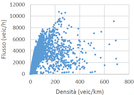
Traveler information systems find it difficult to give people precise advice since road congestion is not well defined, but a traffic status is characterized with a particular pair of values of the fundamental variables. There isn’t a single, unified regulation as of yet [33]. However, there is a vast amount of data on traffic observations, and the phenomenon of traffic is widely recognized. The sole purpose of the example that follows is to serve as an instructive explanation of the ideas behind the fuzzy method that is described in the paper. As is widely known, direct traffic data show two distinct trends in the flow-density plane (Figure. 1a): The flow displays a very noisy and dense structure throughout the range of higher values of density, with an average declining tendency as the density increases. In the range of low levels of density, the flow is practically linear with density and presents few deviations from the average speed. It is commonly recognized that the high-density regime is typified by erratic flow conditions that are dictated by the microscopic mechanism that underlies the traffic stream. These fluctuations include even minor driving movements that result in a stop-and-go traffic pattern.

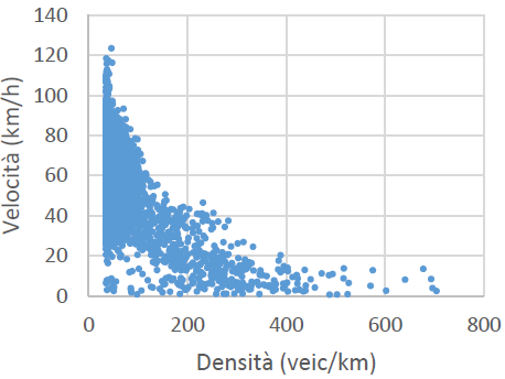
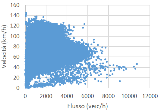
Figures 1a, 1b and 1c illustrate a 15-min observation of the traffic of one of the sections for several months and it is evident from the figures that collecting traffic data for a long period continuously introduces a huge noisy component. The scope of the proposed model is to simulate the general state of the road and derive a relation-ship between the fundamental variables by applying the fuzzy Mamdani inference approach regardless of their value [33]. Each part has been modelled and executed independently because they could each have a distinct general state. The network consists of two main branches: the North (Highway) and the South (Tangential), the results of which are provided in Section 4.

3. Methodology

A traffic stream can be characterized by its current state and the change in its condition. To identify in which state the traffic is in, congestion should be quantified and detected how it is spreading. From this point of view, this paper is an evaluation of the average situation of traffic process in the related time interval as an index between [0-1]. The main purpose is to answer the questions what is happening, and how critical is the current situation in terms of congestion condition level which reflects the severity of traffic. It has been built with a fuzzy model in MATLAB.

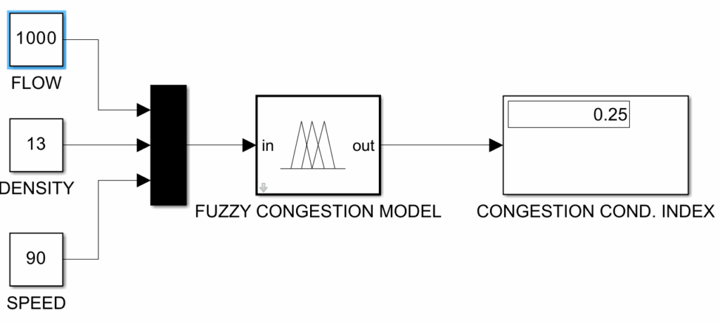
The fuzzy model named ‘Fuzzy Congestion Model’, represented in the middle of the Figure 2, computes the average congestion level by using average flow, average density, and average speed information. All input and output variables have been defined by setting linguistic terms which help us represent them with a wide range. We set n_x1 = n_x2 = n_x3 = 5 linguistic terms as:

$$F = \{FF, RFF, AF, CF, VCF\},$$

$$K = \{VLD, LD, MD, HD, VHD\},$$

$$V = \{VS, S, A, F, VF\}.$$

The output variable is also classified as:

$$CCI = \{VL, L, M, H, VH\}$$

Explanation of variables are: FF: Free Flow, RFF: Reasonably Free Flow, AF: Average Flow, CF: Congested Flow and VCF: Very Congested Flow, VLD: Very Low Density, LD: Low Density, MD: Medium Density, HD: High Density and VHD: Very High Density, VS: Very Slow, S: Slow, A: Average, F: Fast and VF: Very Fast, VL: Very Low, L: Low, M: Medium, H: High and VH: Very High.

While linguistic definitions give the variables a thinking and understanding way to close humans, they need to represent numerically. In order to complete the process, all variables are converted from crisp numbers into membership degrees of the fuzzy set, or fuzzified. Membership functions are utilized in this process, providing the numerical value’s degree of belongingness to the associated fuzzy set inside a closed interval [0,1]. Here, 1 expresses full membership and 0 states non-membership. In this paper, triangular membership (Equation 5) functions are used, since they are one of the most used examples and they are effective in reflecting the characteristics of the fuzzy sets used here.

$$\mu(x) = \begin{cases}
0,\, x \leq amin \text{ or } x \geq amax \\
\frac{x – amin}{\beta – amin},\, x \in (amin, \beta) \\
\frac{amax – x}{amax – \beta},\, x \in (\beta, amax)
\end{cases}\tag{5}$$

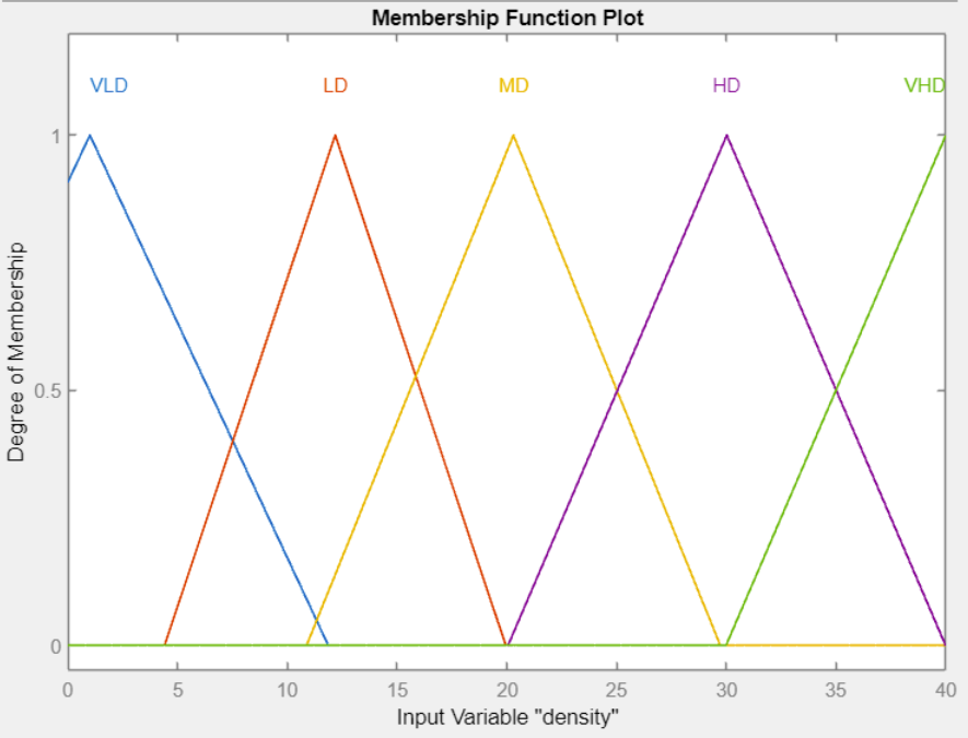
As an example of the mathematical form, the membership function of the Medium level of Density (MD) variable is provided in Eq. 6 and its demonstration is given with Figure 3.

$$\mu_{MD}(k) = \begin{cases}
0,\, k \leq 11 \text{ or } k \geq 30 \\
\frac{k – 11}{20 – 11},\, x \in (11, 20) \\
\frac{30 – k}{30 – 20},\, x \in (20, 30)
\end{cases}\tag{6}$$

Figure 3 shows the membership function plots of the density input variable. All the Very Low, Low, Medium, High, and Very High-density levels are the set members of K. Hence, the MD is a set member of the K fuzzy set. It has a membership degree of K fuzzy set that Eq. 6 gives us. This means it has a certain quantity of numerical belongingness to the K fuzzy set. That numerical value in [0-1] is calculated by Eq. 6.

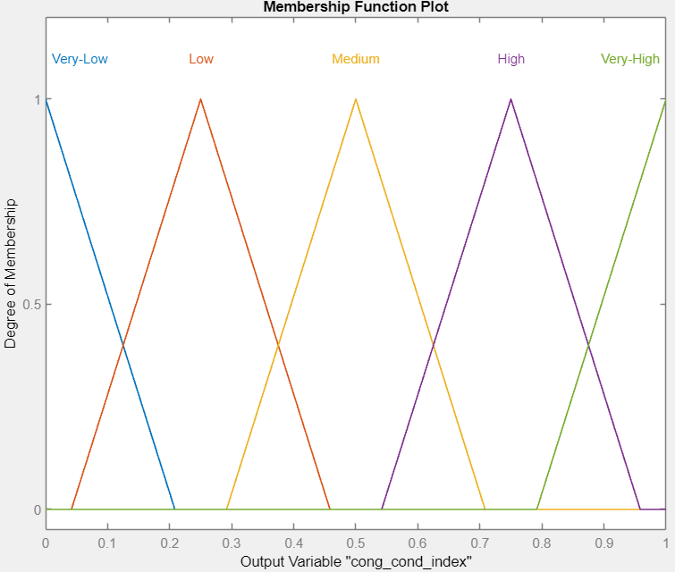
Similarly, Figure 4 shows the membership function plots of congestion condition level index output variable. In both plots (Figure 3 and 4), the horizontal plane shows the value range of the related variables, while the vertical plane gives the membership function value of it in the range [0-1]. The range intervals of the related variables are set after a close investigation according to the data. It is to note that the terms are imprecisely defined following the fuzzy logic concept, and there are no clear cuts between the fuzzy congestion levels.

The fundamental aspect of the approach is to represent the input-output connection, which shows how input variables reflect onto the output universe, in order to construct the nonlinear surface model and make an inference. We define 45 rules for this application and they can be stated mathematically as:

$$(F \cdot F(f)) \odot_{\min} (K \cdot K(k)) \odot_{\min} (V \cdot V(v)) \rightarrow (A \cdot A(f, k, v))$$

where the symbol • states the linguistic term is, symbol \(\Theta_{\min}\) states the logic operator AND. Some of fuzzy if-then rules are given in Table 1 below. 45 rules have been modelled for this application.

Table 1: If-then rules for congestion condition index

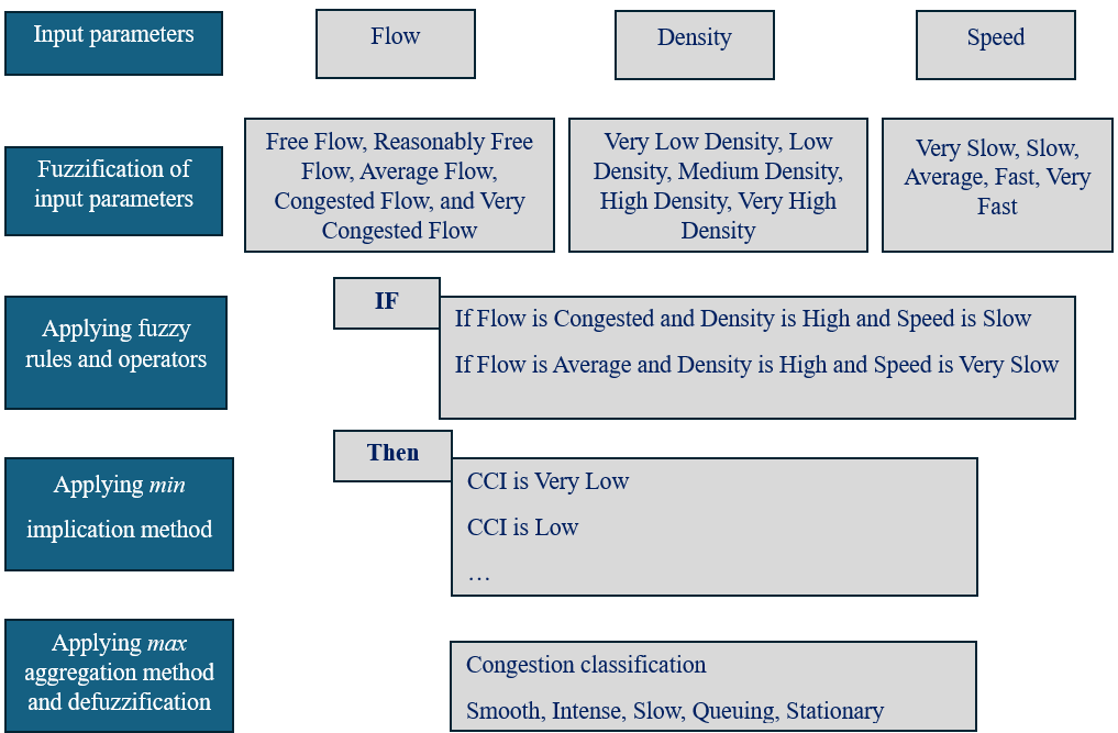
The framework of the method is given in Figure 5. The figure shows the structure of the model, with input parameters, assigned linguistic variables to our crisp inputs, applied fuzzy rules and operators, chosen implication and aggregation method as well as calculated value of congestion as a defuzzied output.

Detailed information about methodological steps such as variable definitions, fuzzification, rules formulations and defuzzification can be seen in [36].

4. Application Results

The main scope of this study is to identify the traffic condition ranges of Padua-Venice motorway network, which is composed by 4 branches of 3-lane roads with separate carriageways, the motorway has a total length of about 74 km and 16 intersections. Real traffic data collected from 31st December 2018 to the 30th of August 2019 contains the following information: local unit code, code section counting, day type, road (section) id, date, flow, density, and harmonic speed aggregated every 15 minutes. The whole data was examined statistically section-by-section; however, it is important to mention that, due to temporary failures of some detectors, some parts of the data are missing. We have neglected them in the application step. In this research, we investigated the congestion from Monday through Saturday for eight months, during the hours of 6:30 am to 9:00 am. The application is run on MATLAB fuzzy logic toolbox R2020b and SIMULINK.

4.1. Traffic situation in the motorway (Northern part)

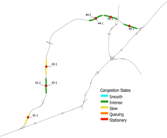
The first step of the application consisted in computing the speed predictions for 15-minute time intervals between 6:30-9:00 for all sections along the northern part of the network. Table 2 shows the congestion levels with average observed intervals, and Figure 6 depicts the traffic condition for all sections of the motorway.

A similar pattern, with intense or slow state levels, may be seen in the observations of traffic states with average intervals along the entire freeway. At section 43, the change to a slow traffic status is smooth. Sections 42 and 44, on the other hand, move to a more intensive condition. The point at which an intense condition transitions to a slow state is reached when flows exceed 1400 cars per hour and density passes 17 vehicles per kilometres.

Table 2: Traffic state results with average observed intervals

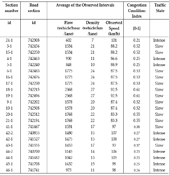
In this case, the average speed decreases by around 15% from its previous level. This means that drivers can drive at around 67% of the free-flow speed level of the road. In such a traffic state, flow and density rates decrease to around 1150 vehicles/h and 14 vehicles/km, respectively. This allows the speed level to grow up to around 106.0 km/h, which equals more than 75% of its free-flow level, and it gives drivers more freedom to manoeuvre. There is no severe congestion and no Stationary state along the highway with this subset of data, because having an average level of flow and low level of density allows Fast level of speed with a high membership and Average and Very Fast levels of speed with low memberships, so this situation occurs in an Intense state generally. It was coloured in Figure 6.

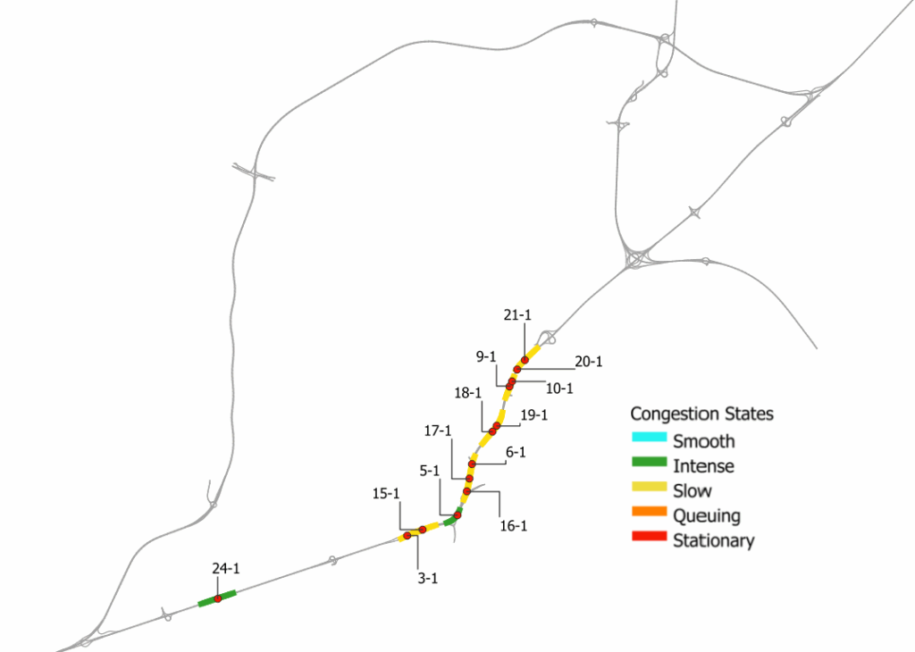
4.2. Traffic situation in the highway (Tangential part)

The same computations have been done for all sections in the Tangential part of the network as well. This application is run with the same subset of data with 5-minute time intervals to criticize the effectiveness of the timeframe in characterizing the trend of rate changes. The observations of traffic states with average intervals all along the highway show a similar pattern, with intense or slow state levels. However, after having an intense situation, there is a clear transition to a slow state at sections 3 and 15 with an almost double amount of congestion indices. In this case, the average levels of flow and density go up to 2.5 and 3 times higher than the previous section’s levels and that intensity causes a medium congestion and it is classified in the next congested state by the proposed model. Like the motorway part, there is no severe congestion and no Stationary state along the highway, as vehicles can move in a Fast level of Speed with a range between 85.5 km/h to 101km/h with a low membership, so this situation occurs in a slow state generally. Identified traffic states have been colored in Figure 7.

5. Discussion and Conclusion

5.1. Evaluation of congestion index by the fuzzy congestion calculator with flow, density, and speed variables

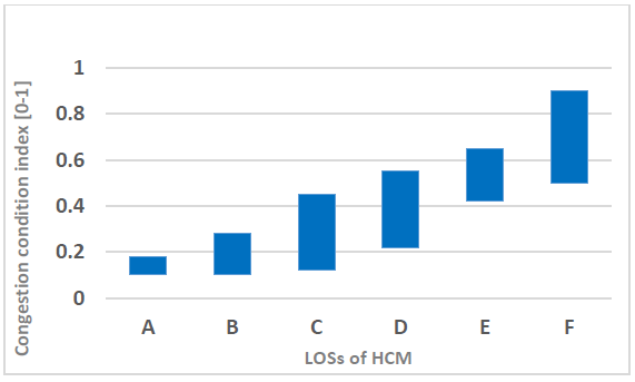
Table 3 summaries the results in evaluating congestion condition index (CCI) for some selected intervals of the field data including variables for density, speed, and flow. The intervals are chosen at random so that the traffic conditions encompass the entire spectrum of the traffic level index. The following lists the LOSs established by the Highway Capacity Manual [37] are shown for comparison. The detailed comparison with the LOSs was given in the next section.

Here, Table 3’s observation (with a focus on average values) enables the following important conclusions to be drawn:

• Table 3 demonstrates that there is a comparatively large variation of density for the same speed. For instance, the densities for the sampling numbers 8, 9, 17, 24, and 99 at the speed level with v = 88-89 (km/h) are 8, 20, 18, 42, and 22 (veh. /lane/km), respectively.
• Similarly, there is a comparatively large range in speed for a given value of density. For instance, sample numbers 46, 52, and 89 have a speed range of [118–77] (km/h) for density k = 31 (veh./lane/km), but their flow range (veh./lane/hr) is rather wide (3588, 495, 375). These show that the traffic state cannot be adequately represented by a single variable.
• Additionally, Table 3 demonstrates the speed is not highly responsive to density alone at the “Very Low” and “Low” levels. For densities k = 2, 3, and 12, the corresponding average speeds (veh./lane/km) are 111.3, 106.4, and 99.0 (km/h). Speed drops by only 11.05% as densities rise six times from 2 to 12 (veh./lane/km). While the flow increases along with the density, the speed also reduces dramatically. For instance, when the flow hits 1800–2000 (veh. /lane/hr), as in indices of 69, 73, and 89, speed drops 26.6% to the level of 73–77 (km/h). This corroborates the idea that the traffic status is a specific tuple of the basic variables’ values. As such, it requires contemporaneous attention.

The congestion indices generated by the FIS system are displayed in Figure 8 across with the LOS as described by [37]. Despite the fact that LOSs are connected to a comparatively broad range of congestion condition indices (CCIs), Figure 8 illustrates a general correlation between the CCIs and service levels. The CCIs of the various LOSs significantly overlap. It is possible to state that Very Low congestion (µVL = {-0.208 0 0.208}) is mainly linked with LOS A and partially with LOS B in

Table 3: Evaluation results

relation to the fuzzy partitioning of the CCI in Figures. 8 and 4. Low congestion (µL = {0.041 0.25 0.458}) is mostly linked to LOS C, sporadically to LOS B, and barely to LOS A. A little amount of medium congestion (µM = {0.30 0.5 0.708}) is linked to LOS C, and most of it to LOS D and E. Finally, Very High congestion (µVH = {0.791 1 1.208}) is strictly associated with LOS F.

5.2. Comparison with the US Highway Capacity Manual’s Service Level definitions

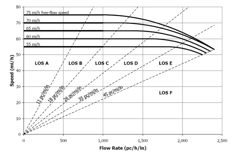
To provide additional insight into the significance of the suggested approach, the outcomes have been contrasted with the similar LOSs estimations derived using the HCM method [37], which establishes service traffic levels using the figure 9 diagram as a basis. Since the HCM speed-flow curves derive from observations conducted in the USA, they should only be used as a means of comparing different approaches and applied very carefully to an Italian motorway. The speed limit on the freeway under investigation is 130 km/h, which is higher than the ranges taken into account by the HCM. On the other hand, a LOS can be applied to the actual traffic states if a projection of the patterns of HCM curves is accepted. This experiment, however, shows that the combined observations of all three state variables are inconsistent with the theoretical model, which focuses on a univariate relationship between flow and speed and the state equation (3). It’s true that if density is taken into account as the LOS identification indicator, then the recorded state of traffic on the road falling between 11 veh/km/lane (18 veh/mi/lane) and 17 veh/km/lane (27 veh/mi/lane) would be classified as either LOS C or LOS D. Nevertheless, the associated LOS will change from LOS B to LOS C if the flow values—which span an array of values from 973 veh/h/lane to 1531 veh/h/lane—are taken into account. More importantly, the density ranges from 7 veh/km/lane to 27 veh/km/lane on the highway would be associated with all levels from A to F with density guidance, while they would be considered in levels B to F for a huge range of flows between 602 veh/h/lane and 2368 veh/h/lane. These traffic conditions were categorized using the fuzzy technique as either slow or intense. The fuzzy method overcomes classification ambiguity caused by inherent mistakes created by the steady-state principles underpinning the HCM methodology and encompasses the inevitable ambiguity of traffic state classification because it takes into account all three state variables at once.

Furthermore, because the qualitative description makes use of common descriptors and is better suited for informing drivers, it is easier than a scale classification. A sensitivity analysis was conducted in terms of the condition of traffic range index between [0-1] to observe the impact of the chosen membership function of the suggested fuzzy model. For that analysis, five cases with triangular, trapezoidal and Gauss, Gaussbell, and Gauss2 function shapes have been carried out and the triangular membership function is stepped out as the best function type [36].

5.3. Conclusion

This article handles the traffic state identification problem and proposes a Mamdani-based fuzzy logic application with a much bigger real dataset from a motorway in Italy. To address the value of multi-dimensional evaluation and we already possess all three-traffic flow variables, we examined the capability of fuzzy reasoning to simulate the relationships between variables and driving behaviour modelling. Moreover, predicted states have been discussed by comparing the LOSs by HCM. The fuzzy technique, which is based on a non-univocal range characterization of traffic circumstances, looks to be a more acceptable strategy for traffic congestion classification because LOS is a stepwise assessment and does not convey a concept of congestion level clearly. Since the fuzzy method considers all three state variables, it takes into account the inevitable uncertainty in traffic state recognition and removes any ambiguity in categorization caused by inaccuracies resulting from the steady-state assumptions that underlie the HCM methodology. Furthermore, because the qualitative description makes use of common descriptors and is better suited for informing drivers, it is more straightforward than a scale classification. When properly designed using rules, the fuzzy-based congestion analyser can be used as a tool to help control actions on expressways under boisterous conditions. The current applications are in places like Singapore and Los Angeles [38-39]. These systems continuously monitor the state of the roads and modify the length of the signals. As a result, traffic flows more smoothly, stop-and-go situations are less frequent, and fuel consumption is decreased. Moreover, some Indian towns are experimenting with fuzzy logic-based systems that enable traffic signal modifications in real-time upon detection of emergency vehicles [40]. This facilitates the clearance of space for emergency vehicles and, by cutting reaction times in urgent situations, may save lives. By incorporating intelligence into traffic management, these solutions enhance effectiveness, security, and environmental sustainability.

However, due to the case study’s static environment, this analysis limited to show severe and/or temporal congestion. For future works, the model will be extended with a consideration of this issues. Additionally, unanticipated events like accidents, weather changes, etc., will be handled to make developing control actions on motorways more convenient.

Conflict of Interest

The authors declare no conflict of interest.

Acknowledgment

This work has not been supported by any foundation.

1. Y. Liu, C. Zhen, D. Huili, “Highway traffic congestion detection and evaluation based on deep learning techniques.” Soft Computing vol. 27, no.17, 12249-12265, 2023, doi.org/10.1007/s00500-023-08821-6.
2. C. Wang, C. Yuting, W. Jie, Q. Jinjin, “An improved crowddet algorithm for traffic congestion detection in expressway scenarios.” Applied Sciences , vol. 13, no. 12, 2023, 7174, doi.org/10.3390/app13127174.
3. T. G. Huang, L. H. Xu, and X. Y. Kuang. “Urban road traffic state identification based on fuzzy C-mean clustering.” Journal of Chongqing Jiaotong University (Natural Science), vol. 34, no. 2, 101-106, 2015.
4. H.W. Liu, Y.T. Wang, X.K. Wang, Y. Liu, Y. Liu, X.Y. Zhang, F. Xiao, “Cloud Model-Based Fuzzy Inference System for Short-Term Traffic Flow Prediction”, Mathematics, vol. 11, no. 11, 2509, 2023, doi.org/10.3390/math11112509.
5. Z. Liu, C. Lyu, Z. Wang, S. Wang, P. Liu, Q. Meng, 2023 “A Gaussian-process-based data-driven traffic flow model and its application in road capacity analysis.” IEEE Transactions on Intelligent Transportation Systems, vol. 24, no. 2, 1544-1563, 2023, doi.org/10.1109/TITS.2022.3223982.
6. K. Zhao, G. Dudu, S. Miao, Z. Chenao, S. Hongbo, “Short-term traffic flow prediction based on VMD and IDBO-LSTM.” IEEE Access 2023, doi.org/10.1109/ACCESS.2023.3312711.
7. J, Ying, “Research on methods of urban road traffic condition identification”, Qingdao Univ. (Eng. Technol. Ed.), vol. 27, no. 3, 84–87, 2012, doi.org/10.1007/978-981-19-1057-9_26.
8. P.H. Bovy, I. Salomon, “Congestion in Europe: Measurements, patterns and policies.” Travel behaviour: spatial patterns, congestion and modelling, 143-179, 2002, doi.org/10.4337/9781781951187.
9. A. Almeida, S. Brás, S. Sargento, I. Oliveira, “Exploring bus tracking data to characterize urban traffic congestion”. Journal of Urban Mobility, vol. 4, 100065, 2023, doi.org/10.1016/j.urbmob.2023.100065.
10. M.A.P. Taylor, “Exploring the nature of urban traffic congestion: concepts, parameters, theories and models.” In Proceedings, 16th Arrb Conference, 9-13 November, Perth, Western Australia, Vol. 16, No. 5. 1992.
11. I. Pedram, S. Salek, R. Omrani, Defining and Measuring Urban Congestion—Guidelines for Defining and Measuring Urban Congestion, Transportation Association of Canada: Ottawa, ON, Canada. 2017, Access (December 2020).
12. ECM, The spread of congestion in Europe, 11th Round Table on Transport Economics, OECD Publication Service, 1999.
13. M. Aftabuzzaman, “Measuring traffic congestion – a critical review”, Proceedings of the 30th Australasian Transport Research Forum, 16, 2007.
14. J. Xia, W. Huang, J. Guo, “A clustering approach to online freeway traffic state identification using ITS data”, KSCE Journal of Civil Engineering, vol. 16, 426-432, 2012, doi 10.1007/s12205-012-1233-1.
15. B. Priambodo, A. Azlin, A.K. Rabiah, “Prediction of average speed based on relationships between neighbouring roads using K-NN and neural network.”, 18-33, 2020, doi.org/10.3991/ijoe.v16i01.11671.
16. N. Tilahun, P. Thakuriah, “Incorporating weather information into real-time speed estimates: Comparison of alternative models”, J. Transp. Eng., vol. 139, no.4, 379–389, 2012, doi.org/10.1061/(ASCE)TE.1943-5436.0000506.
17. L. Zhang, J. Ma, X. Liu, M. Zhang, X. Duan, Z. Wang, “A novel support vector machine model of traffic state identification of urban expressway integrating parallel genetic and C-means clustering algorithm”, Tehnički vjesnik, vol. 29, no. 3, 731-741, 2022, doi.org/10.17559/TV-20211201014622.
18. Y. Zhu, Y. Zheng, “Retracted article: traffic identification and traffic analysis based on support vector machine.” Neural Computing and Applications, vol. 32, no. 7, 1903-1911, 2020, doi.org/10.1007/s00521-019-04493-2.
19. S. Dong, “Multi class SVM algorithm with active learning for network traffic classification.” Expert Systems with Applications vol. 176, 114885, 2021, doi.org/10.1016/j.eswa.2021.114885.
20. D. Mladenović, S. Janković, S. Zdravković, S. Mladenović, A. Uzelac, “Night traffic flow prediction using K-nearest neighbors algorithm”, Operational research in engineering sciences: theory and applications, vol. 5, no. 1, 152-168, 2022, doi.org/10.31181/oresta240322136m.
21. F. Harrou, Z. Abdelhafid, S. Ying, “Traffic congestion monitoring using an improved kNN strategy.” Measurement, vol. 156, 107534, 2020, doi.org/10.1016/j.measurement.2020.107534.
22. T. Seo, T. Kusakabe, Y. Asakura, “Calibration of fundamental diagram using trajectories of probe vehicles: Basic formulation and heuristic algorithm”, Transportation Research Procedia, vol. 21, 6-17, 2017, doi.org/10.1016/j.trpro.2017.03.073.
23. C.G. Claudel, A.M. Bayen, “Guaranteed bounds for traffic flow parameters estimation using mixed Lagrangian-Eulerian sensing,” 46th Annual Allerton Conference on Communication, Control, and Computing, 636–645, 2008, doi.org/10.1109/ALLERTON.2008.4797618.
24. J. Jiang, N. Dellaert, T. Van Woensel, L. Wu, “Modelling traffic flows and estimating road travel times in transportation network under dynamic disturbances”, Transportation, vol. 47, 2951-2980, 2020, doi.org/10.1007/s11116-019-09997-3.
25. G.B. Whitham, Linear and Nonlinear Waves, Wiley-Interscience, 1974.
26. R. Pradhan, S. Shrestha, D. Gurung, “Mathematical modeling of mixed-traffic in urban areas.” Mathematical modeling and computing, vol. 9, No. 2, 226-240, 2022, doi: 10.23939/mmc2022.02.226.
27. A. Iftikhar, Z.H. Khan, T.A. Gulliver, K.S. Khattak, M.A. Khan, M. Ali, N, Minallahe, “Macroscopic traffic flow characterization at bottlenecks”, Civil Engineering Journal, vol. 6, no. 7, 1227-1242, 2020, doi.org/10.28991/cej-2020-03091543.
28. J. Junfeng, H. Wang, “Traffic behavior recognition from traffic videos under occlusion condition: a Kalman filter approach.” Transportation research record, vol. 2676, no. 7, 55-65, 2022, doi.org/10.1177/03611981221076426.
29. F. Zheng, S.E. Jabari, H.X. Liu, D. Lin, “Traffic state estimation using stochastic Lagrangian dynamics”, Transportation Research Part B: Methodological, vol. 115, 143-165, 2018, doi.org/10.1016/j.trb.2018.07.004.
30. Y. Liu, Z. Cai, H. Dou, “Highway traffic congestion detection and evaluation based on deep learning techniques”, Soft Comput, vol. 27, no. 20, 12249–12265, 2023, https://doi.org/10.1007/s00500-023-08821-6.
31. A. Nantes, D. Ngoduy, A. Bhaskar, M. Miska, E. Chung, “Real-time traffic state estimation in urban corridors from heterogeneous data”, Transportation Research Part C: Emerging Technologies, vol. 66, 99-118, 2016, doi.org/10.1016/j.trc.2015.07.005.
32. C. Wang, W. Zhang, C. Wu, H. Hu, H. Ding, W. Zhu, “A traffic state recognition model based on feature map and deep learning” Physica A: Statistical Mechanics and its Applications, vol. 607, 128-198, 2022, doi.org/10.1016/j.physa.2022.128198.
33. T.D. Toan, Y.D. Wong, “Fuzzy logic-based methodology for quantification of traffic congestion”, Physica A: Statistical Mechanics and its Applications, vol. 570, p.125784, 2021, doi.org/10.1016/j.physa.2021.125784.
34. A. Skabardonis, P. Varaiya, K.F. Petty, “Measuring recurrent and nonrecurrent traffic congestion”, Transportation Research Record, vol. 1856, no. 1, 118-124, 2003, doi.org/10.3141/1856-12.
35. Erdinç, G., Colombaroni, C. and Fusco, G., “Two-stage fuzzy traffic congestion detector”, Future transportation, vol.3, no. 3, 840-857, 2023, doi.org/10.3390/futuretransp3030047.
36. G. Erdinç, C. Colombaroni, G. Fusco, “Application of a Mamdani-Based Fuzzy Traffic State Identifier to a Real Case Study”, In 2023 8th International Conference on Models and Technologies for Intelligent Transportation Systems (MT-ITS) 1-6, IEEE, 2023, doi.org/10.1109/MT-ITS56129.2023.10241428.
37. National Academies of Sciences, Engineering, and Medicine, Highway Capacity Manual 7th Edition: A Guide for Multimodal Mobility Analysis, Washington, DC: The National Academies Press, 2022, doi.org/10.17226/26432.
38. G. Hewei, A.S. Sadiq, M.A. Taheir, “Adaptive fuzzy-logic traffic control approach based on volunteer IoT agent mechanism”, SN Computer Science, vol. 3, no. 1, p.68, 2022, doi.org/10.1007/s42979-021-00956-3.
39. B. Yulianto, “Adaptive Traffic Signal Control Using Fuzzy Logic Under Mixed Traffic Conditions”, Proceedings of the 5th International Conference on Rehabilitation and Maintenance in Civil Engineering. ICRMCE 2021. Lecture Notes in Civil Engineering, vol 225. Springer, Singapore, doi.org/10.1007/978-981-16-9348-9_59.
40. A. Agrahari, M.M. Dhabu, P.S. Deshpande, A. Tiwari, M.A. Baig, A.D. Sawarkar, “Artificial Intelligence-Based Adaptive Traffic Signal Control System: A Comprehensive Review”, Electronics, vol.13, no. 19, p.3875, 2024, doi.org/10.3390/electronics13193875.

Citations by Dimensions

Citations by PlumX

Crossref Citations

This paper is currently not cited.

No. of Downloads per Month

No. of Downloads per Country