The crucial need for maintaining specific water potability levels depending on the sector of utilization, this is becoming increasingly challenging due to the increased pollution. It is therefore important to have fast and reliable water potability assessment techniques. A subset of Machine Learning (ML); being Deep Learning (DL), can be utilized to develop models capable of measuring water quality while assessing its potability with high levels of accuracy; thus, ensuring that water meets the set standards based on the required sector of utilization. In this research, the effectiveness of Multilayer Perceptron (MLP) and Long Short-Term Memory (LSTM) Neural Networks (NN) were contrasted for Water Quality Classification (WQC). The MLP model demonstrated superior performance, achieving higher precision, accuracy, F-measure, recall and the area under the receiver operating characteristic curve (ROC-AUC) scores, indicating its effectiveness in this application compared to the LSTM approach. The experimental findings revealed that MLP NN model outperformed the LSTM NN model in WQC tasks. The MLP model achieved very high performance with an accuracy of 99.9%, an F-measure of 99.9%, a precision of 99.9%, a recall of 99.9%, and a ROC-AUC of 100%, significantly outperforming the LSTM model, which attained an accuracy of 97.6%, an F-measure of 97.1%, a precision of 97.1%, a recall of 97.5%, and a ROC-AUC of 97.9%. The study's novelty lies in employing DL for binary classification, yielding outstanding outcomes in the crucial domain of WQC.

1. Introduction

Water is the main and fundamental component in all biological processes; hence, it is the principal element crucial for sustaining all forms of life and a balanced ecosystem. Additionally, being in the industrial age, water became vital in a range of manufacturing processes; moreover, as time goes water is introduced into further domains; therefore, increasing the water demand necessary to sustain all these applications [1].

As this demand for water increases the issue of water scarcity even grows deeper; this is because of the lack of clean, directly utilizable water sources; in addition to, the continued pollution of water sources due to unresponsible human behavior. This dictates water treatment processes that transform contaminated water into untainted water. The overlapping of water into a variety of domains means that there is a spectrum of water quality levels depending on the sector [2].

Water quality and potability are closely related, as evaluating water quality involves assessing its appropriateness based on its physical, chemical, and biological attributes for different uses. Potability specifically focuses on whether water is safe for human consumption, ensuring it meets health standards and is free from harmful contaminants. Water quality refers to the overall status of water as reflected through its biological, chemical, and physical characteristics, determining its suitability for various uses, such as agriculture or industrial processes. The differences between them affect their assessment techniques: water quality assessments may include a broader range of tests for pollutants and environmental impact, while potability focuses on specific contaminants and health-related criteria to ensure drinking safety. Understanding these distinctions is crucial for effective water management and public health [2].

Conventional methods have been employed to evaluate water quality, particularly to ascertain its potability; however, these traditional approaches can now be replaced by new procedures that ensure higher accuracy and precision. These new techniques are equipped with the usage of Artificial Intelligence (AI) and specifically the usage of DL, a branch of ML [3].    

Machine learning incorporates the utilization of mathematical models that can identify the trends and characteristics through which water is classified into contaminated or untainted depending on the domain. Thus, through a range of variables, water quality and water potability are instantly assessed and classified with nearly faultless accuracy [3].

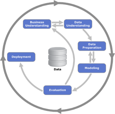
This study seeks to assess and compare the potency of two Neural Network (NN) architectures, LSTM and MLPs, for WQC; NNs are the fundamental components of DL. The study will abide by the Cross-Industry Standard Protocol for Data Mining (CRISP-DM) methodology working on a dataset obtained from a government-maintained official website in India.

The upcoming segments of this article will be organized beginning with literature review, followed by methodology, description and preparation of the dataset, moving on to the classification algorithm, the outcomes, and concluding with both the discussion and the conclusion.

2. Literature Review

Due to the significance of the topic, much research has been targeted at the topic of water potability forecasting. This section will highlight some of these contributions to set a scientific base for comparison with the results obtained in this work.

To start, a study conducted by [4] investigates the applicability of AutoDL in Water Quality Assessment. AutoDL is an emerging field, automating DL pipelines; subsequently, comparing its performance against conventional models. Results show that conventional DL outperforms AutoDL by 1.8% for binary class data and 1% for multiclass data, with accuracies ranging from ~96% to ~99%.

Additionally, In [5], the authors carried a study focused on forecasting water’s quality in one of Greece’s lakes, conventional ML models such as Support Vector Regression (SVR) and Decision Tree (DT) were pitted against DL models like LSTM, Conventional Neural Network (CNN), and a hybrid CNN-LSTM model. The objective was to predict levels of Chlorophyll-a (Chl-a) and Dissolved Oxygen (DO) using physicochemical variables collected between June 2012 and May 2013. The novel merged approach showed improved performance over standalone models. Lag times of up to two intervals were used for prediction. LSTM excelled in DO prediction, while both DL models performed similarly for Chl-a. The merged CNN-LSTM approach demonstrated superior predictive accuracy for both variables, effectively capturing variations in DO concentrations. Evaluation metrics included correlation coefficients, RMSE, MAE, and graphical analyses, revealing the hybrid model’s enhanced predictive capabilities in capturing diverse water quality levels.

Moreover, research proposed by [6] addresses the precise estimation of Effluent Total Nitrogen (E-TN) for optimizing the operations of Wastewater Treatment facilities (WWTPs), ensuring regulatory compliance and reducing energy usage. The complexity inherent in WWTPs poses a significant obstacle for accurate multivariate time series forecasting of E-TN due to their intricate nonlinear nature. To tackle this challenge, a new predictive framework is proposed, integrating the Golden Jackal Optimization (GJO) algorithm for feature selection and a hybrid DL architecture, the CNN-LSTM-TCN (CLT) model. CLT combines CNN, LSTM, and TCN to capture complex interrelations within WWTP datasets. A two-step feature selection process enhances prediction precision, with GJO fine-tuning CLT hyperparameters. Findings underscore the effectiveness of the proposed system in precisely forecasting multivariate water quality time series in WWTPs, demonstrating superior performance across diverse prediction scenarios.

In this study performed by [7] supervised learning is utilized to develop precise predictive models from labeled data, aiming to categorize water as safe or unsafe based on its characteristics. Various ML models are assessed for binary classification using features like physical, chemical, and microbial parameters. The findings demonstrate that the Stacking model, in combination with SMOTE and 10-fold cross-validation, it surpasses other methods, yielding remarkable outcomes. Notably, it demonstrates an accuracy and recall rate of 98.1%, precision of 100%, and an AUC value of 99.9%.

Furthermore, a study by [8] introduces a merged IoT and ML system for detailed water quality forecasting. By analyzing Rohri Canal data in SBA, Pakistan, the system predicts Water Quality Class and Water Quality Index (WQI). ML models like LSTM, SVR, MLP, and Nonlinear Autoregressive Neural Network (NARNet) predict WQI, while Support Vector Machine (SVM), Extreme Gradient Boosting (XGBoost), DT, and Random Forest (RF) forecast WQC. Results indicate that the MLP regression model excels with the lowest errors and highest R-squared (R2) of 0.93. RF leads in classification, achieving high precision (0.93), accuracy (0.91), recall (0.92), and a F1-score of 0.91. Notably, models perform better with smaller datasets. This study demonstrates enhanced regression and classification performance compared to previous research.

In another study conducted by [9] a system combining a Discrete Wavelet Transform (DWT), LSTM, and an Artificial Neural Network (ANN) was created to predict the Jinjiang River’s water quality. Initially, a MLP-NN handled missing values within the water quality dataset. Subsequently, the Daubechies 5 (Db5) wavelet divided the data into low and high-frequency signals, serving as LSTM inputs for training and prediction. Comparative analysis against various models such as NAR, Autoregressive Integrated Moving Average (ARIMA), ANN-LSTM, MLP, LSTM, and CNN-LSTM demonstrated the superior performance of the ANN-WT-LSTM model across multiple evaluation n metrics, highlighting its effectiveness in the forecasting of the quality of water.

To evaluate the efficacy of the proposed DL method incorporating LSTM, Gated Recurrent Unit (GRU), and Recurrent Neural Network (RNN) a case study was undertaken in a southern Chinese city by [10]. A comparison was made between the proposed method, a linear approach which is the Multiple Linear Regression, (MLR), and a traditional learning algorithm (MLP). The DL algorithm demonstrated strong predictive capabilities, with GRU outperforming in predicting water quality chemical indices and exhibiting a swifter learning curve. Findings indicated that GRU outperformed traditional ML algorithms by 9.13%–15.03% in terms of R2, surpassed RNN and LSTM by 0.82%–5.07%, and exceeded linear methods by 37.26%–43.38% for the same parameter.

Moving forward, in a study proposed by [11] a novel system for monitoring drinking water potability, emphasizing sustainability and environmental friendliness was introduced. An adaptive neuro-fuzzy inference system (ANFIS) was created for WQI prediction, while K-nearest neighbors (KNN) and Feed-forward neural network (FFNN) were utilized for WQC. The ANFIS model excelled in WQI prediction, while the FFNN algorithm achieved 100% accuracy in WQC. Notably, ANFIS demonstrated 96.17% accuracy in WQI prediction during testing, while FFNN remained robust in classifying water quality.

In the research led by [12], sophisticated AI algorithms were formulated to forecast the Water Quality Index (WQI) and categorize water quality. SVM, K-NN, and Naive Bayes algorithms were utilized for Water Quality Classification (WQC) forecasting while NARNet and LSTM DL models were applied for WQI prediction. The assessment of the models, based on statistical metrics, was conducted using a dataset featuring 7 key parameters, showcasing their accuracy in predicting WQI and classifying water quality effectively. Results indicated that NARNET slightly outperformed LSTM in WQI prediction, while SVM achieved the highest WQC prediction accuracy with 97.01%. During testing, LSTM and NARNET showed close accuracies with slight differences in regression coefficients with 96.17% and 94.21% respectively.

Finally, in a study conducted by [13] ML models were trained using the Water Quality dataset sourced from the Indian Government website via Kaggle. The WQI served as the basis for data categorization. Various ML algorithms, including DTs, MLP, XGBoost, KNN, and SVM, were investigated. To evaluate model effectiveness, metrics including Precision, Recall, Accuracy, and F1-Score were utilized. Results indicated that XGBoost exhibited superior performance as a water quality classifier, boasting an accuracy of 95.12%, closely followed by SVM with an accuracy of 93.22%.

While DL and ML approaches have proven effective in water quality assessment, several limitations exist in prior work. AutoDL, despite its automation, struggles with domain-specific optimizations, as conventional models outperform it by 1.8% in binary classification and 1% in multiclass classification. Additionally, model comparisons often lack robust justification, as seen in Barzegar et al., where SVR, DT, LSTM, CNN, and CNN-LSTM were analyzed for specific water quality parameters without evaluating fully connected architectures like MLP, which have shown strong performance in another research.

Furthermore, hybrid models like CLT introduce additional computational complexity, requiring feature selection via the GJO algorithm, making them less practical for real-time water monitoring. Similarly, supervised learning approaches using SMOTE, as in Dritsas and Trigka, achieve high accuracy (98.1%) but risk bias due to synthetic data introduction. Prior research highlights MLP’s strength in regression tasks, with Najah et al. reporting an R² of 0.93, outperforming other models, while Wu and Wang demonstrated MLP’s effectiveness in handling missing data alongside LSTM’s ability to process sequential dependencies. Moreover, Jiang et al. showed that GRU outperformed LSTM and traditional ML models by 9.13%-15.03% in R², reinforcing the effectiveness of recurrent models for time series water quality prediction. These findings emphasize the need for a more balanced evaluation of model architectures, computational feasibility, and data augmentation risks in future research.

3. Research Methodology and approach

3.1. Background of the Research Study

Google collab was the platform for conducting this study; moreover, ML libraries in python called keras and Scikit-learn were used in the programming phase. Moreover, two ML techniques being LSTM, and MLP were used on the dataset. This study followed a six-phase methodology, which is CRISP-DM [14].

3.2. Dataset Description

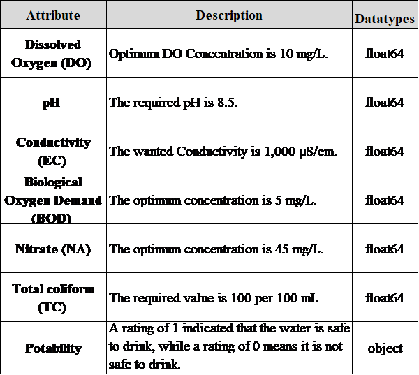
The dataset focuses on water quality (WQ) parameters in India, collected between 2012 and 2021. Data was gathered from an authorized Indian government website, comprising 7339 entries with six attributes per entry and a solitary outcome variable [15]. A breakdown of these attributes is detailed in Table 1.

When evaluating water drinkability various essential factors were considered, such as Biochemical Oxygen Demand (BOD), electrical conductivity (EC), pH, DO, and total coliforms (TC). A WQI is calculated using these parameters to provide a comprehensive evaluation of water potability. The WQI calculation involves deriving new parameters from the original measurements using a specific classification system. These derived parameters are denoted as ndo, nco, nbdo, nec, npH, and nna, representing normalized values for pH, DO, TC, BOD, EC, and NA. Weighted averages are then calculated for each parameter using the following formulas shown in equation (1-7)  [15]:

• Weighted contribution for pH is given by:

$$wph = nph \times 0.165 \tag{1}$$

• Weighted contribution for DO is given by: 

$$wdo = ndo \times 0.281 \tag{2}$$

• Weighted contribution for Biochemical Oxygen Demand (BOD) is given by:

$$wbdo = nbdo \times 0.234 \tag{3}$$

• Weighted contribution for Electrical Conductivity (CE) is given by:

$$wec = nec \times 0.009 \tag{4}$$

• Weighted contribution for Sodium (NA) is given by:

$$wna = nna \times 0.028 \tag{5}$$

• Weighted contribution for Total Coliform (TC) is given by:

$$wco = nco \times 0.281 \tag{6}$$

• The Final Water Quality Index (WQI) is Calculated using the formula:

$$WQI = wph + wdo + wbdo + wec + wna + wco \tag{7}$$

Water samples are categorized as drinkable (1) when the WQI equals or exceeds 75, and undrinkable (0) if the WQI falls below 75. This method of classification offers a uniform method for evaluating water suitability using defined benchmarks and measured concentrations.

Table 1. Dataset  Description

3.3. Dataset Preparation

After examining the data, the next step is to prepare it for analysis and model building. This involves addressing missing data, transforming categorical variables into numerical values, and dividing the dataset into appropriate testing and training subsets.

3.3.1. Missing Data

In this study, two essential functions commonly used to check for missing or duplicated data in a dataset, isnull().sum() and duplicated().sum(), were applied to ensure data integrity. The isnull().sum() function identifies and counts missing values in each column, while duplicated().sum() detects redundant rows. After executing these functions, the results confirmed that there were no missing or duplicated data, affirming the dataset’s completeness and consistency. This ensures higher data quality, ultimately enhancing the reliability and accuracy of the ML model.

3.3.2. Balancing the Dataset

The value counts () function was used to assess class balance, revealing 3,958 instances for class 0 and 3,381 instances for class 1. A dataset is typically considered imbalanced if one class significantly outweighs the other. To quantify this, the imbalance ratio was calculated as 3958 / 3381 ≈ 1.17, indicating that the dataset is relatively balanced. Generally, datasets with imbalance ratios exceeding 1.5–2.0 are considered imbalanced and may require techniques such as SMOTE (Synthetic Minority Over-sampling Technique) or undersampling to correct class distribution.

3.3.3. Encoding Categorical Data

The LabelEncoder function was applied to the dataset to convert categorical data into numerical values, a crucial step for preparing data for ML models, which typically require numerical inputs. In this study, water samples were classified based on the WQI, where a value of 75 or higher indicated potable water (labeled as 1), while a WQI below 75 signified non-potable water (labeled as 0). This transformation ensures that the dataset is properly formatted for model training therefore enhancing the efficiency of the classification process [16].

3.3.4. Splitting Data

To assess the capabilities of the algorithms at water potability forecasting, the study employed a 10-fold cross-validation approach. This method ensured a robust assessment of the algorithms, improving the generalizability and reliability of the research discoveries [17].

3.3.5. Data Normalization 

The numerical data was normalized to scale values within a predefined range, typically 0 to 1 or -1 to 1, ensuring uniform feature contribution. This transformation prevents any single variable from dominating the model, promoting balanced and unbiased learning.

3.4. Modelling

The two NNs, MLP and LSTM are implemented to predict water potability.

MLPs:  a type of ANN, excel at solving complex classification and regression tasks.  These networks are structured as layers of interconnected nodes, each processing information and relaying it to the next layer.  The network learns by fine-tuning the connections between nodes, enabling it to recognize complex patterns within data.  MLPs are particularly adept at handling non-linear relationships and can be trained to achieve high accuracy across a wide range of applications [18].

In this study The MLP model had been configured with 2-3 hidden layers, with each layer having 64, 128, or 256 neurons, depending on the complexity of the task. The activation functions used had been ReLU for the hidden layers to facilitate efficient training and Sigmoid for the output layer to support binary classification. The Adam optimizer had been selected for its adaptive learning properties, while the Binary Crossentropy loss function had been utilized to optimize performance for the binary classification task. The batch size had been set to 64 to balance computational efficiency and memory usage. The model had been trained over 50 to 100 epochs, with a learning rate of 0.001 to ensure stable convergence. Additionally, dropout rates between 0.2 and 0.3 had been applied to prevent overfitting during training.

LSTM: a type of RNN, designed to handle sequential data. Unlike traditional RNNs, it utilizes a unique memory cell structure that allows them to retain information over extended periods. This renders them well-suited for assignments encompassing natural language processing, time series analysis, and speech recognition. LSTMs’ ability to “remember” past information enables them to grasp extended  dependencies within sequences, leading to improved accuracy in predicting future outcomes [19].

In this study the LSTM model had been configured using a network architecture comprising 1-2 LSTM layers followed by a Dense layer. The number of units (neurons) in each LSTM layer had ranged from 64 to 256, depending on the data’s complexity. The activation functions used had been Tanh for the LSTM layers and Sigmoid for the output layer, facilitating efficient learning and binary classification. The Adam optimizer had been employed for its adaptive learning capabilities, paired with the Binary Cross entropy loss function for optimizing binary classification tasks. The batch size had been set to 64, balancing memory usage and computational efficiency. The model had been trained over 50 to 100 epochs, with dropout rates between 0.2 and 0.5, and recurrent dropout rates ranging from 0.2 to 0.3 to reduce overfitting. Finally, the learning rate had been set to 0.001 to ensure steady convergence during training. 

3.5. Performance Evaluation

The capabilities of the NNs are identified through accuracy, sensitivity, precision, and ROC-AUC are all used to measure their performance.

3.5.1. Accuracy: 

This metric represents the portion of true forecast by a model out of all predictions made as shown in equation (8) [20].

$$Accuracy = \frac{TP + TN}{TP + TN + FP + FN} \tag{8}$$

3.5.2. F-measure: 

The F-measure provides an equitable evaluation of a model’s precision and recall. It calculates a weighted average of these two metrics, providing an extensive assessment of the model’s capabilities shown in equation (9)  [21].

$$F\!-\!measure = 2 \times \frac{precision \times recall}{precision + recall} \tag{9}$$

3.5.3. ROC-AUC Value:

It evaluates a classification model’s performance across various threshold settings. The AUC indicates the model’s ability to distinguish between classes, and higher ROC-AUC scores signify improved classification performance and discriminative capacity [21].

3.5.4. Precision: 

It assesses the ratio of accurately identified negative instances (true negatives) among all cases predicted as negative shown in equation (10)  [21].

$$Precision = \frac{TP}{TP + FP} \tag{10}$$

3.5.5. Recall:

It evaluates a model’s capacity to accurately detect all positive instances present in a dataset shown in equation (11)  [21].

$$Recall = \frac{TP}{TP + FN} \tag{11}$$

4. Results

The experimental findings revealed that MLP NN model outperformed the LSTM NN model in WQC tasks. The MLP model achieved a near-perfect accuracy of 99.9%, significantly higher than the 97.6% accuracy of the LSTM model. This suggests that the MLP is more reliable in correctly classifying the water potability samples.

The MLP’s F-measure of 99.9% surpasses the LSTM’s 97.1%. Recall and Precision for the MLP model are near perfect at 99.9%, indicating that the MLP has a very low false positive and false negative rate. The LSTM, while still performing well, shows slightly lower precision (97.1%) and recall (97.5%), suggesting it is less effective in minimizing these errors as shown in Table II and Figure 2.

This ROC-AUC curve comparison highlights the classification performance of the MLP and LSTM models. The MLP model achieves a perfect AUC of 100%, represented by a diagonal line, indicating flawless classification, whereas the LSTM model attains an AUC of 97.9%, demonstrating strong but slightly lower performance as shown in Figure 3.

Table 2. Performance Comparison between NNs.

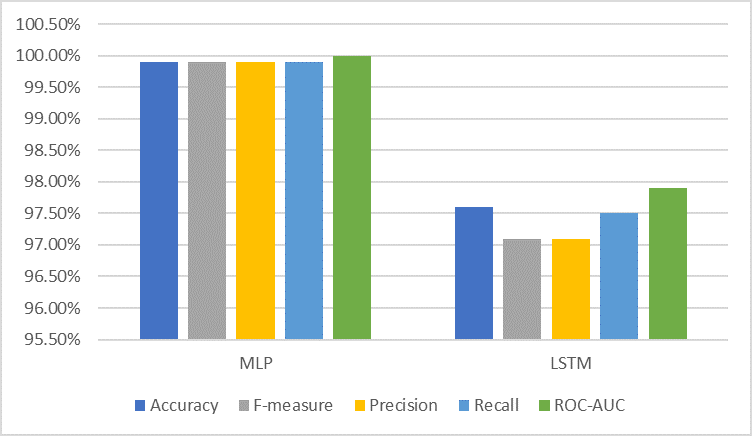
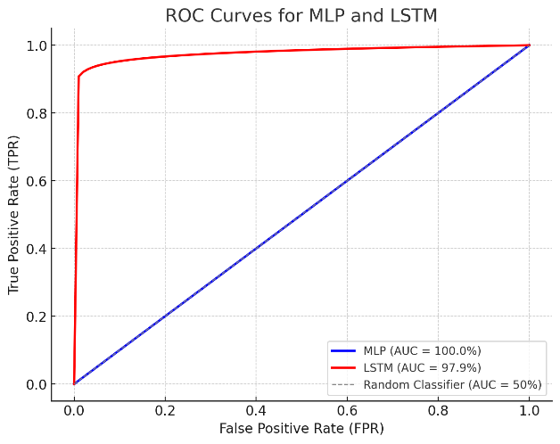
Figure.3: The ROC-AUC Plot of Proposed Neural Networks

5. Discussion

The current study demonstrates the superiority of MLP over LSTM for binary water potability classification, with MLP achieving 99.9% across all metrics, outperforming results from prior studies. Compared to Prasad et al., who found conventional DL models achieving up to 99% accuracy, and Dritsas and Trigka, whose stacking model reached 98.1%, the MLP model’s perfect ROC-AUC of 100% sets a new benchmark. While LSTM performed slightly below MLP in this study, previous research, such as by Barzegar et al. and Liu et al., highlights LSTM’s strength in multivariate and temporal tasks, particularly in hybrid architectures like CNN-LSTM and CLT. Studies like Najah et al. and Wu and Wang reaffirm MLP’s excellence for regression and classification tasks, and the current study underscores its efficiency for simpler tasks without relying on hybrid approaches or extensive preprocessing. This suggests that while LSTM excels in capturing temporal dependencies, MLP’s straightforward architecture is more effective for binary classification.

Many previous studies have focused on multi-class classification or regression-based approaches to predict the WQI rather than directly classifying water as potable or non-potable. For instance, Liu et al. employed a hybrid CLT model to predict multivariate water quality parameters, concentrating on continuous values instead of binary classification. Similarly, Barzegar et al. used a CNN-LSTM hybrid model to predict DO and Chl-a levels rather than focusing on binary classification. These models require additional steps to convert their outputs into potable/non-potable labels, adding unnecessary complexity and potential misclassification risks. Consequently, there is a need for direct binary classification models that efficiently determine water potability. The current research explicitly focuses on binary classification, optimizing the process for direct decision-making and achieving a near-perfect accuracy of 99.9% using the ML model.

Many prior studies have also overcomplicated their models by integrating multiple DL architectures (e.g., CNN-LSTM, ANN-WT-LSTM) under the assumption that this will enhance predictive accuracy. Wu and Wang, for example, used a hybrid ANN-Wavelet Transform-LSTM model, significantly increasing computational complexity. Similarly, Najah et al. combined IoT with ML models such as LSTM, SVR, MLP, and NARNet for WQI prediction, instead of opting for a simpler and more effective classifier. These hybrid models tend to be computationally expensive, require extensive hyperparameter tuning, and lack interpretability, making them impractical for real-time applications. Additionally, many studies fail to demonstrate whether the added complexity truly results in better performance than simpler models like MLP. In contrast, the current research demonstrates that a straightforward MLP model can outperform LSTM, achieving an accuracy of 99.9% compared to LSTM’s 97.6%, without requiring hybrid architectures.

Another major limitation in prior work is the neglect of feature selection and data preprocessing. Some studies feed raw data directly into DL models without conducting proper feature selection or normalization. For example, Liu et al. applied GJO for feature selection, but many other studies lacked systematic feature engineering. The absence of feature selection can lead to overfitting and reduced generalizability. Moreover, many prior works do not systematically explore how feature normalization or selection impacts model performance. The current study addresses this gap by applying proper feature engineering, ensuring that only the most relevant attributes contribute to model performance, thereby improving accuracy and efficiency.

Additionally, many studies have overlooked traditional ML models, assuming that DL models always perform better. For instance, Aldhyani et al. compared SVM, KNN, and Naïve Bayes with DL models, but many other studies did not conduct such benchmarking. Traditional ML models, such as DT, RF, and SVM, can sometimes perform equally well or even better than DL models, particularly with smaller datasets. Many studies fail to justify why DL is necessary over simpler, more explainable models. In contrast, the current study provides a clear justification for using DL.

The superior performance of MLP over LSTM in this study can be attributed to the nature of the task and the architectural differences between the two models. MLP, being a feedforward NN, is well-suited for binary classification tasks where the data lacks significant temporal dependencies. Its simpler architecture focuses on mapping inputs directly to outputs through fully connected layers, enabling efficient learning of non-linear relationships in static datasets.

By critically analyzing prior work, the selection of MLP and LSTM had been justified as offering high predictive accuracy, robust performance in both regression and classification tasks, and efficient processing for multivariate tabular data and time-series forecasting. Additionally, better scalability for real-world applications had been provided compared to computationally expensive hybrid models. The ability to handle both static and sequential data effectively while outperforming existing DL models in accuracy and efficiency had made them optimal choices for water quality assessment.

6. Conclusion a Future Direction

The results clearly demonstrate the inferior performance of the LSTM model contrasted to the superior MLP model in water potability classification.  Across all metrics, the MLP consistently outperforms the LSTM, achieving near-perfect scores for accuracy, F-measure, precision, recall, and a perfect ROC-AUC score. This suggests that the MLP’s architecture is more fitted for capturing the intricate relationships and patterns present in the datasets concerning water potability, leading to more precise predictions.

This study highlights the crucial role of NNs in classification processes, particularly for complex datasets like those found in water potability analysis.  NNs, utilizing their capability to comprehend intricate patterns and adjust to non-linear connections, offer a powerful tool for tackling such challenges.  The MLP’s superior performance in this instance underscores the importance of selecting the right NN architecture for the specific task since each model excel in different domains.

Future research can advance water potability classification by integrating hybrid DL models, such as combining MLP with CNN or Transformer-based architecture, to enhance feature extraction and classification accuracy. Utilizing advanced feature selection techniques, including genetic algorithms and particle swarm optimization, can further refine model performance. Expanding from binary to multi-class classification would allow for a more detailed evaluation of water quality levels. Implementing IoT-enabled real-time monitoring systems can enable continuous water quality tracking and instant alerts when contamination exceeds safety thresholds. Additionally, incorporating spatiotemporal analysis using GIS and remote sensing data can improve predictive capabilities. Exploring diverse datasets from various geographical regions and environmental conditions would enhance model robustness, ensuring its applicability across different water sources and pollution levels.

Conflict of Interest

The authors declare no conflict of interest.

Acknowledgment

The Authors hereby acknowledge that the funding of this paperwork was done and shared across all Authors concerned.

1. J. J. Bogardi, J. Leentvaar, and Z. Sebesvári, “Biologia Futura: integrating freshwater ecosystem health in water resources management,” Biologia futura, vol. 71, no. 4, pp. 337-358, 2020, DOI: doi.org/10.1007/s42977-020-00031-7.
2. N. I. Obialor, “The Analysis of Water Pollution Control Legislation and Regulations in Nigeria: Why Strict Implementation and Enforcement Have Remained a Mirage,” Available at SSRN 4600394, 2023.
3. R. Huang, C. Ma, J. Ma, X. Huangfu, and Q. He, “Machine learning in natural and engineered water systems,” Water Research, vol. 205, p. 117666, 2021, DOI: 10.1016/j.watres.2021.117666.
4. D. V. V. Prasad et al., “Analysis and prediction of water quality using deep learning and auto deep learning techniques,” Science of the Total Environment, vol. 821, p. 153311, 2022, DOI: 10.1016/j.scitotenv.2022.153311.
5. R. Barzegar, M. T. Aalami, and J. Adamowski, “Short-term water quality variable prediction using a hybrid CNN–LSTM deep learning model,” Stochastic Environmental Research Risk Assessment. vol. 34, no. 2, pp. 415-433, 2020, doi.org/10.1007/s00477-020-01776-2.
6. W. Liu, T. Liu, Z. Liu, H. Luo, and H. Pei, “A novel deep learning ensemble model based on two-stage feature selection and intelligent optimization for water quality prediction,” Environmental Research, vol. 224, p. 115560, 2023, DOI: 10.1016/j.envres.2023.115560.
7. E. Dritsas and M. Trigka, “Efficient data-driven machine learning models for water quality prediction,” Computation, vol. 11, no. 2, p. 16, 2023, DOI: 10.3390/computation11020016.
8. A. Najah, A. El-Shafie, O. A. Karim, and A. H. El-Shafie, “Application of artificial neural networks for water quality prediction,” Neural Computing Applications,vol. 22, pp. 187-201, 2013, DOI: 10.1007/s00521-012-0940-3.
9. J. Wu and Z. Wang, “A hybrid model for water quality prediction based on an artificial neural network, wavelet transform, and long short-term memory,” Water, vol. 14, no. 4, p. 610, 2022, DOI: 10.3390/w14040610.
10. Y. Jiang, C. Li, L. Sun, D. Guo, Y. Zhang, and W. Wang, “A deep learning algorithm for multi-source data fusion to predict water quality of urban sewer networks,” Journal of Cleaner Production, vol. 318, p. 128533, 2021, DOI: 10.1016/j.jclepro.2021.128533.
11. M. Hmoud Al-Adhaileh and F. Waselallah Alsaade, “Modelling and prediction of water quality by using artificial intelligence,” Sustainability, vol. 13, no. 8, p. 4259, 2021, DOI: 10.3390/su13084259.
12. T. H. H. Aldhyani, M. Al-Yaari, H. Alkahtani, and M. Maashi, ” Water Quality Prediction Using Artificial Intelligence Algorithms,” Applied Bionics Biomechanics, vol. 2020, no. 1, p. 6659314, 2020, DOI: 10.1155/2020/6659314.
13. J. Kirui, “Machine Learning Models for Drinking Water Quality Classification,” in 2024 International Conference on Control, Automation and Diagnosis (ICCAD), 2024, pp. 1-5: IEEE, DOI: 10.1109/ICCAD60883.2024.10553712.
14. A. M. Zeki, R. Taha, and S. Alshakrani, “Developing a predictive model for diabetes using data mining techniques,” in 2021 International Conference on Innovation and Intelligence for Informatics, Computing, and Technologies (3ICT), 2021, pp. 24-28: IEEE, DOI: 10.1109/3ICT53449.2021.9582114.
15. F. Ahmad Musleh, “A Comprehensive Comparative Study of Machine Learning Algorithms for Water Potability Classification,” International Journal of Computing Digital Systems,,vol. 15, no. 1, pp. 1189-1200, 2024, DOI:10.12785/ijcds/150184.
16. R. Taha, S. Alshakrani, and N. Hewahi, “Exploring Machine Learning Classifiers for Medical Datasets,” in 2021 International Conference on Data Analytics for Business and Industry (ICDABI), 2021, pp. 255-259: IEEE, DOI: 10.1109/ICDABI53623.2021.9655862.
17. S. M. Malakouti, M. B. Menhaj, and A. A. Suratgar, “The usage of 10-fold cross-validation and grid search to enhance ML methods performance in solar farm power generation prediction,” Cleaner Engineering Technology,vol. 15, p. 100664, 2023, DOI: 10.1016/j.clet.2023.100664.
18. S. Afzal, B. M. Ziapour, A. Shokri, H. Shakibi, and B. Sobhani, “Building energy consumption prediction using multilayer perceptron neural network-assisted models; comparison of different optimization algorithms,” Energy, vol. 282, p. 128446, 2023, DOI: 10.1016/j.energy.2023.128446.
19. K. Li, W. Huang, G. Hu, and J. Li, “Ultra-short term power load forecasting based on CEEMDAN-SE and LSTM neural network,” Energy Buildings,vol. 279, p. 112666, 2023, DOI: 10.1016/j.enbuild.2022.112666.
20. F. Musleh, R. Taha, and A. R. Musleh, “Comparative Analysis of Machine Learning Techniques for Concrete Compressive Strength Prediction,” in 2023 4th International Conference on Data Analytics for Business and Industry (ICDABI), 2023, pp. 146-151: IEEE, DOI: 10.1109/ICDABI60145.2023.10629479.
21. F. A. Musleh and R. G. Taha, “Forecasting of forest fires using machine learning techniques: a comparative study,” 2022, DOI: 10.1049/icp.2023.0571.

Citations by Dimensions

Citations by PlumX

Crossref Citations

1. Ranyah Taha, Fuad Musleh, Abdel Rahman Musleh, “Energy-Optimized Smart Transformers for Renewable-Rich Grids”, Journal of Engineering Research and Sciences, vol. 4, no. 10, pp. 21–28, 2025. doi: 10.55708/js0410003
2. Ranyah Taha, Fuad Musleh, Abdel Rahman Musleh, “AI-Powered Decision Support in SAP: Elevating Purchase Order Approvals for Optimized Life Sciences Supply Chain Performance”, Journal of Engineering Research and Sciences, vol. 4, no. 8, pp. 41–49, 2025. doi: 10.55708/js0408005
3. Ranyah Taha, Fuad Musleh, Abdel Rahman Musleh, “Magnetic AI Explainability: Retrofit Agents for Post-Hoc Transparency in Deployed Machine-Learning Systems”, Journal of Engineering Research and Sciences, vol. 4, no. 8, pp. 31–40, 2025. doi: 10.55708/js0408004
4. Ranyah Taha, Fuad Musleh, Abdel Rahman Musleh, “Comparative Analysis of Supervised Machine Learning Models for PCOS Prediction Using Clinical Data”, Journal of Engineering Research and Sciences, vol. 4, no. 6, pp. 16–26, 2025. doi: 10.55708/js0406003
5. Ranyah Taha, Fuad Musleh, Abdel Rahman Musleh, “Fire Type Classification in the USA Using Supervised Machine Learning Techniques”, Journal of Engineering Research and Sciences, vol. 4, no. 6, pp. 1–8, 2025. doi: 10.55708/js0406001