This article addresses the calculation of approximation errors in numerical methods for solving differential equations. A fundamental challenge when replacing differential equations with discrete representations is ensuring that the discrete solution closely approximates the exact solution. To tackle this, a grid area is established for the difference solution, with discrete solutions evaluated at specific nodal points. Traditionally, the degree of approximation in this context is expressed using the notation , where h represents the grid step and p indicates the order of accuracy. A significant advancement in this area is the application of the moving nodes method, which enables the calculation of approximation errors at these nodal points. This method allows researchers to derive an approximate analytical expression for the discrete solution, which serves as a foundation for calculating the approximation error.

1. Introduction 

This article is an expanded version of the article presented in [1]. The numerical solution methods for differential equations fundamentally rely on transforming differential problems into difference problems [2–5]. In simpler terms, solving differential equations requires understanding how to approximate them. This involves converting a differential equation into a system of algebraic equations, which is based on the values of the desired functions at specific points on a grid. Recent studies [6]–11] have introduced a new approach for approximating differential operators, enhancing the accuracy and efficiency of these methods. One of the significant advantages of the moved node method is that it enables the calculation of an explicit expression for the approximation error when replacing differential equations with difference ones. Understanding this error is crucial because it provides insights into the reliability and accuracy of the numerical solution. By quantifying the error, researchers can refine their methods and improve the overall quality of the numerical solutions obtained.

In conclusion, the transformation of differential equations into difference equations is a fundamental aspect of numerical analysis. The development of innovative methods like the moved node method represents a significant advancement in this field, providing researchers and practitioners with powerful tools to tackle complex differential problems more effectively. As numerical methods continue to evolve, the importance of understanding and minimizing approximation errors will remain a critical area of focus for ensuring the accuracy and reliability of solutions.

On the basis of the movable node, an approximate analytical expression for the difference solution of the differential problem was obtained [12]. This development represents a significant step forward in numerical methods, as it provides a more refined approach to approximating solutions to differential equations. The analytical expression derived from the movable node approach allows for greater flexibility and accuracy when dealing with complex differential problems.

In [13], the moving nodes method was further applied to construct the control volume method, which is widely used in computational fluid dynamics and other engineering applications.

In [14], the authors explored the potential to increase accuracy by combining the moving nodes method with the ideas of Richardson’s extrapolation. Richardson’s extrapolation is a technique used to improve the precision of numerical approximations by utilizing solutions obtained at different grid resolutions. By integrating this method with the moving nodes approach, it is possible to achieve higher-order accuracy in the numerical solutions, thereby reducing the error associated with the approximation.

Some questions regarding the monotonicity of the difference scheme using the movable node are addressed in [15]. Monotonicity is an important property in numerical methods, as it ensures that the numerical solution behaves in a physically realistic manner, avoiding non-physical oscillations or spurious solutions. Understanding and ensuring the monotonicity of the difference scheme is crucial for maintaining the stability and reliability of the numerical method, especially in problems involving sharp gradients or discontinuities.

The application of the moving nodes method to various applied problems is reflected in [16]. This demonstrates the versatility of the method across different fields, such as fluid dynamics, heat transfer, and structural analysis.

Moreover, based on the choice of the velocity profile on the edge of the control volume, qualitative schemes were obtained in [17]. The velocity profile plays a critical role in determining the flow characteristics and behavior within the control volume.

In summary, the integration of the movable node method into various numerical frameworks and its application to real-world problems highlights its significance in advancing numerical analysis. The ongoing exploration of its properties, such as accuracy, monotonicity, and adaptability to different contexts, continues to enhance the capability of numerical methods in solving complex differential equations effectively. As research in this area progresses, the potential for further innovations and improvements remains substantial, promising even greater advancements in the field of numerical solutions.

This paper describes the application of the moving nodes method to the calculation of the approximation error. The moving nodes method provides a dynamic approach to numerical analysis, allowing for the adjustment of grid points based on the behavior of the solution.

When a two-point boundary value problem is solved using difference methods, the question of the degree of approximation typically arises. This degree of approximation is crucial as it directly impacts how closely the numerical solution aligns with the exact solution. In numerical analysis, understanding the closeness of the exact solution to its approximation is essential for evaluating the effectiveness of the chosen method.

The quality of the difference scheme is often assessed based on this degree of approximation. A higher degree indicates a more accurate representation of the solution, while a lower degree suggests potential discrepancies that may arise from the numerical method employed. This evaluation is typically conducted by analyzing the behavior of the approximation error, which quantifies the difference between the exact solution and the numerical approximation.

Interestingly, in this analysis, other parameters—such as the coefficients of the differential equation—are not explicitly involved in the expression for the approximation error. This is significant because it allows researchers to focus on the fundamental aspects of the numerical method without being distracted by the specific characteristics of the differential equation being solved. By isolating the approximation error from these coefficients, the analysis can yield more generalized insights into the behavior of the numerical solution.

Obtaining an explicit expression allows researchers to identify how changes in the grid size, the choice of the moving nodes, and other factors influence the accuracy of the numerical solution. Furthermore, it enables the development of strategies to minimize the approximation error, thus enhancing the overall quality of the numerical method.

By utilizing the moving nodes method to derive this explicit expression, the paper contributes to a deeper understanding of the approximation error in the context of two-point boundary value problems. This understanding is crucial for advancing numerical methods, as it provides a foundation for improving accuracy and reliability in solving complex differential equations. Ultimately, the insights gained from this analysis can inform future research and applications, paving the way for more effective numerical solutions in various scientific and engineering fields.

When a two-point boundary value problem is solved by difference methods, the question of the degree of approximation usually appears. For the closeness of the exact and approximation of the solution, and the quality of the difference scheme are evaluated based on the degree of this parameter. With such an analysis, other parameters (the coefficients of the differential equation) are not explicitly involved in the approximation error expression. Obtaining an explicit expression for the approximation error makes it possible to analyze it.Consider the simplest ordinary differential equation with boundary conditions

$$\frac{d^{2}u}{dx^{2}} = C, \quad u(0)=0, \; u(1)=1\tag{1}$$

where C is constant.
Create a uniform grid on segments [0,1] with step h. A uniform grid on a segment x∈[0,1] with step h has the form:

$$\overline{\omega}_h = \{x_k = hk, \; k = 0,1,\ldots,N, \; h \cdot N = 1\}$$

Let us replace the second-order derivative by the difference relation [18]:

$$\frac{U_{i+1} – 2U_i + U_{i-1}}{h^2} = C, \quad 1 \leq i \leq N-1, \; U_0=0, \; U_N=1\tag{2}$$

Difference scheme (2) traditionally has order O(h)². However, if we solve system (2) by the Tomas algorithm, we obtain a numerical solution that coincides with the exact analytical solution for any grid steps h at the grid nodes. Those. scheme (2) approximates (1) exactly.

2. Method For Determining Approximation Error

Let we have a differential equation

$$Lu = f , \tag{3}$$

where L is a differential operator, f is a known function, and u is an unknown function. (3) the equation is considered in some domain D with appropriate boundary conditions. The differential equation (3) is replaced by the difference equation [18] :

$$L_hu_h = f_h , \tag{4}$$

where L_h is the difference operator, u_h is the unknown grid function, and f_h is the approximation of the function f at the grid nodes.

Usually, the approximation error is given as [18,19]:

$$Q_h = L_h [u]_h – f_h , \tag{5}$$

where [u]_h is the exact solution of (3) at the grid nodes. Using the Taylor series, from (5) one obtains that, Q_h = O(h^m), where h is the grid step and m is the degree of approximation.

You can determine an explicit approximation error if you use the method of a moving node, which allows you to extend the definition to the entire area D. This allows you to introduce an approximation error like this:

$$R_h = L_h \{u\}_h – f_h. \tag{6}$$

Here {u}_h is a predefined continuous function by means of a moveable node. Approximate calculation of the approximation error of type (6) is demonstrated using simple examples.

3. Results and Discussion

As an application of the above approach, consider examples.

3.1. Simple Boundary Value Problem

Consider a simple boundary value problem:

$$\frac{d^2u}{dx^2} = f(x), \quad u(0)=u_a, \; u(1)=u_b \tag{7}$$

Let’s build a non-uniform grid on segments [0,1]:

$$\overline{\omega}_h = \{0 = x_0 < x_1 < \dots < x_{N-1} < x_N = 1, \; k=0,1,\dots,N\}$$

In the non-uniform grid, we replace (7) with the difference problem:

$$\frac{2}{x_{i+1}-x_{i-1}} \left( \frac{U_{i+1}-U_i}{x_{i+1}-x_i} – \frac{U_i-U_{i-1}}{x_i-x_{i-1}} \right) = f(x_i), \quad i=1,2,\dots,N-1. \tag{8}$$

Here U_i is the grid solution of the problem. From here

$$U_i = \frac{U_{i+1}(x_i – x_{i-1}) + U_{i-1}(x_{i+1} – x_i)}{x_{i+1} – x_{i-1}} – \tfrac{1}{2} f(x_i)(x_i – x_{i-1})(x_{i+1} – x_i), \quad i=1,2,\dots,N-1. \tag{9}$$

We redefine the value of the function at non-nodal points as follows. To do this, we consider in (9) \(x_{i+1}, \; x_{i-1}, \; U_{i-1}, \; U_{i+1},\) to be fixed, and x_i to be moved, and the function f(x) to be smooth. Thus, we will complete the grid function on each segment \((x_{i-1}, \; x_{i+1})\).

From (9) we get

$$U_i”(x_i) = -\tfrac{1}{2} f”(x_i)(x_{i+1}-x_i)(x_i-x_{i-1}) – f'(x_i)(x_{i+1}+x_{i-1}-2x_i) + f(x_i) \tag{10}$$

Then the approximation error for the nodal points looks like this:

$$R_h(x_i) = -\tfrac{1}{2} f”(x_i)(x_{i+1}-x_i)(x_i-x_{i-1}) – f'(x_i)(x_{i+1}+x_{i-1}-2x_i) \tag{11}$$

If the grid is uniform for the approximation error, we obtain the expression

$$R_h(x_i) = -\tfrac{1}{2} f”(x_i) h^2, \quad i=1,2,\dots,N-1. \tag{12}$$

If on the segments \((x_{i-1}, \; x_{i+1})\) the function constant approximation error is identically equal to zero and we get the exact solution.

Based on expression (10), the following conclusion can be drawn.

Given a two-point boundary value problem

$$\frac{d^2u}{dx^2} = f^*(x), \quad u(0)=u_a, \; u(1)=u_b$$

and f^*(x) can be represented as

$$f^*(x_i) = -\tfrac{1}{2} f”(x_i)(x_{i+1}-x_i)(x_i-x_{i-1}) – f'(x_i)(x_{i+1}+x_{i-1}-2x_i) + f(x_i)$$

then the difference scheme

$$\frac{2}{x_{i+1}-x_{i-1}} \left( \frac{U_{i+1}-U_i}{x_{i+1}-x_i} – \frac{U_i-U_{i-1}}{x_i-x_{i-1}} \right) = f(x_i), \quad i=1,2,\dots,N-1,$$

gives a grid solution coinciding with the exact solution at the nodal points.

If there is only one internal node point (the node being moved is one), then an approximate analytical solution can be obtained. Indeed, if we rewrite scheme (8) for one moving node, we have

$$2 \left( \frac{U_b – U(x)}{1-x} – \frac{U(x) – U_a}{x} \right) = f(x_i). \tag{13}$$

From here we obtain an approximate analytical solution:

$$U(x) = U_b x + U_a (1-x) – \tfrac{1}{2} f(x_i)(1-x)x. \tag{14}$$

In this case, (14) represents the exact solution of the problem (7) if we put

$$f^*(x) = -\tfrac{1}{2} f”(x)(1-x)x – f'(x)(1-2x) + f(x).$$

The form of the approximation error (11) allows the construction of new schemes of the collocation type. Indeed, if in problem (8) we replace the right side by the expression

$$f(x_i) + A(x_i – x_{i-1})(x_{i+1} – x_i),$$

Here A is still an unknown constant. Parameter A is determined so that the approximation error (11) for a uniform step at node x_i is equal to zero, i.e. collocation type scheme. Then we have

$$A = \tfrac{1}{4} f”(x_i)$$

3.2. Boundary value problem for convection and diffusion equation

Consider a stationary equation in which only convection and diffusion are present without a source.

$$\varepsilon u” + u’ = 0, \tag{15}$$

with boundary conditions v(0) = 0, v(1) =1.

There are various schemes for the difference solution (15) [6, 7]. Based on the moving node technique [1,2], it is possible to explicitly express local errors in the approximation of differential equations. Using the moving node method [1], we will show the efficient calculation of local approximation errors for the model problem (15).

3.1.1. Scheme with central-difference approximation of the convective term

Take a segment \([x_{i-1}; \; x_{i+1}]\) and any point . Consider the grid analog (15)

$$\frac{2\varepsilon}{x_{i+1}-x_{i-1}} \left( \frac{u_{i+1}-u}{x_{i+1}-x} – \frac{u-u_{i-1}}{x-x_{i-1}} \right) + \frac{u_{i+1}-u_{i-1}}{x_{i+1}-x_{i-1}} = 0 \tag{16}$$

At \(x = \tfrac{(x_{i+1} – x_{i-1})}{2},\) we have a central difference approximation. Here, \(u_{i+1}\) is the approximate value of the solution at the point \(x_{i+1}, \; u_{i-1}\) is the approximate value of the solution at the point \(x_{i-1}\).

From (16) we find

$$u = \frac{1}{2\varepsilon(x_{i+1}-x_{i-1})} \Big[ (x-x_{i-1})(2\varepsilon+x_{i+1}-x)u_{i+1} + (x_{i+1}-x)(2\varepsilon-x+x_{i-1})u_{i-1} \Big] \tag{17}$$

From here we get,

$$u’ = \frac{2\varepsilon + x_{i+1} + x_{i-1} – 2x}{2\varepsilon} \cdot \frac{u_{i+1}-u_{i-1}}{x_{i+1}-x_{i-1}}, \tag{18}$$

$$u” = -\frac{1}{\varepsilon} \cdot \frac{u_{i+1}-u_{i-1}}{x_{i+1}-x_{i-1}}. \tag{19}$$

If the difference solution at nodal points is known, then formula (17) makes it possible to determine the unknown at points that are not nodal.

Using formulas (18) and (19), the derivatives are restored at any point of the segment. Multiplying (19) by and adding with (18), we obtain

$$\varepsilon u” + u’ = \Psi_1, \tag{20}$$

where

$$\Psi_1 = \frac{x_{i+1} + x_{i-1} – 2x}{2\varepsilon} \cdot \frac{u_{i+1} – u_{i-1}}{x_{i+1} – x_{i-1}},$$

Equation (20) can be called a differential analog of the difference equation (16); difference equation (16) is a collocation-type scheme.

Using (19), the approximation error can be written as

$$\Psi_1 = -\frac{x_{i+1} + x_{i-1} – 2x}{2} u”.$$

Then equation (20) takes the form

$$\left( \varepsilon + \frac{x_{i+1} + x_{i-1} – 2x}{2} \right) u” + u’ = 0. \tag{21}$$

Thus, difference equation (16) exactly approximates differential equation (21) on the segment \([x_{i-1}, \; x_{i+1}]
\).

Comparison of Eqs. (15) and (21) shows that when Eq. (15) is approximated by scheme (16), scheme diffusion appears with a variable coefficient \(\frac{x_{i+1} + x_{i-1} – 2x}{2}.\)

3.2.2. Upwind Scheme.

Let us consider the difference analog of equation (15), in which the convective term is approximated by the one-sided difference relation 

$$\frac{2\varepsilon}{x_{i+1}-x_{i-1}} \left( \frac{u_{i+1}-u}{x_{i+1}-x} – \frac{u-u_{i-1}}{x-x_{i-1}} \right) + \frac{u_{i+1}-u}{x_{i+1}-x} = 0. \tag{22}$$

From here we get

$$u = \frac{(x-x_{i-1})(2\varepsilon+x_{i+1}-x)u_{i+1} + 2\varepsilon(x_{i+1}-x)u_{i-1}}{(x_{i+1}-x_{i-1})(2\varepsilon+x-x_{i-1})} \tag{23}$$

Determine the first and second derivatives:

$$u’ = \frac{2\varepsilon(2\varepsilon+x_{i+1}-x_{i-1})}{(2\varepsilon+x-x_{i-1})^2} \cdot \frac{u_{i+1}-u_{i-1}}{x_{i+1}-x_{i-1}}, \tag{24}$$

$$u” = \frac{-4\varepsilon(2\varepsilon+x_{i+1}-x_{i-1})}{(2\varepsilon+x-x_{i-1})^3} \cdot \frac{u_{i+1}-u_{i-1}}{x_{i+1}-x_{i-1}} \tag{25}$$

Let us calculate the approximation error

$$\Psi_2 = \frac{2\varepsilon(x-x_{i-1})(2\varepsilon+x_{i+1}-x_{i-1})}{(2\varepsilon+x-x_{i-1})^3} \cdot \frac{u_{i+1}-u_{i-1}}{x_{i+1}-x_{i-1}} \tag{25a}$$

The differential analog of scheme (22) has the form

$$\left( \varepsilon + \frac{x-x_{i-1}}{2} \right) u” + u’ = 0. \tag{26}$$

those. with a scheme against the flow, we have a scheme diffusion with a coefficient . Based on (23) – is a hyperbola, which is monotone on the segment, i.e. scheme (22) is monotonic.

Based on the form of the differential analogue (26), we can conclude that the differential equation

$$\left( \varepsilon + \tfrac{x}{2} \right) u” + u’ = 0 \tag{27}$$

is exactly approximated by the scheme

$$2\varepsilon \left( \frac{u_b – u}{1-x} + \frac{u – u_a}{x} \right) + \frac{u_b – u}{1-x} = 0 \tag{28}$$

Those. solving (28) with respect to u, we obtain the exact solution of differential equation (27).

3.3. Parametric Schemes

In this case, an attempt is made to create a special parametric scheme in order to improve the quality of the circuit. The peculiarity of this approach is the choice of the parameter, which is carried out on the basis of the calculated approximation error, which allows more accurately adjusting the parameters of the scheme to achieve the best indicators. We demonstrate the effectiveness of this method using examples of problems related to convection-diffusion processes, where the correct choice of parameters is especially important for the stability and accuracy of the solution. Consider the problem [19,20].

$$Pe \frac{du}{dx} = \frac{d^2u}{dx^2} + Pe \cdot S(x), \quad u(0)=u_0, \; u(1)=u_1, \tag{29}$$

Here Pe is the Peclet number, S(x) is the source, u is the unknown function.

When problem (29) is discredited, it is essential to approximate the convective term [4]. The standard finite-difference scheme against the flow on a three-point template is:

$$Pe \frac{U – U_W}{x – x_W} = \frac{2}{x_E – x_W} \left( \frac{U_E – U}{x_E – x} – \frac{U – U_W}{x – x_W} \right) + Pe \cdot S(x), \tag{30}$$

Consider the parametric scheme

$$Pe \frac{U – U_W}{x^k – x_W^k} \cdot kx^{k-1} = \frac{2}{x_E – x_W} \left( \frac{U_E – U}{x_E – x} – \frac{U – U_W}{x – x_W} \right) + Pe \cdot S(x), \tag{31}$$

The choice of the parameter k can be found by numerical experiment. Based on the calculated approximation error Rh, it is not difficult to select the parameter k. The idea of approximating the convective term is as follows. We introduce an intermediate variable y(x), and based on the calculation of the derivative of a complex function, we have

$$\frac{du}{dx} = \frac{du}{dy} \cdot \frac{dy}{dx}.$$

For the function y(x) we take a monotonically increasing function, for example, \(y = x^k \cdot \frac{du}{dy}\) will be replaced by the difference relation upstream. Making the assumption that with such a replacement, the approximation error decreases. In this way

$$\frac{du}{dx} \approx \frac{u – u_W}{x^k – x_W^k} \cdot kx^{k-1}.$$

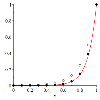
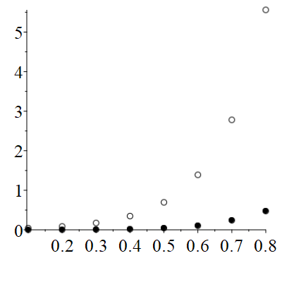
Figure 1 shows the results of calculations \((Pe = 0, \; S(x) = 0, \; N = 11, \; u_0 = 0, \; u_1 = 1),\) at k = 1 and k = 9.

Thus, by carefully choosing the parameter k, we are able to obtain a result that is as close as possible to the exact solution of the problem. This approach allows us to significantly increase the accuracy and reliability of calculations, minimizing approximation errors and ensuring more stable behavior of the numerical method.

3.3. Iterative method to get a solution

It is known that after replacing the differential equation with discrete ones, we obtain a system of algebraic equations [4,5,19,20]. There are two approaches to solving systems of algebraic equations: exact methods and iterative methods. Using the idea of constructing iterative methods for systems of discrete equations, we will show the possibilities of an analytical approximate solution based on the method of moving nodes.

Consider problem (29). If there is only one moving node, approximating the convective term by the upstream scheme from (31) we get (u₀ = 0, u₁ = 1)

$$u^1 = \frac{2x}{2 + Pe(1-x)} + \frac{x(1-x)}{2 + Pe(1-x)} \cdot S(x) \tag{32}$$

This expression is taken as the initial approximation of problem (29). Let’s find the approximation error

$$R^1 = \frac{d^2 u^1}{dx^2} – Pe \frac{du^1}{dx} + Pe \cdot S(x) \tag{33}$$

Let’s calculate the second approximation

$$u^2 = u^1 + \omega x(1-x)R^1$$

Find the approximation error R² .

$$R^2 = \frac{d^2 u^2}{dx^2} – Pe \frac{du^2}{dx} + Pe \cdot S(x)$$

Thus, we carry out an iterative process in the form

$$u^k = u^{k-1} + \omega x(1-x)R^{k-1} + Pe \cdot S(x), \quad k = 2,3,\dots \tag{34}$$

In (34) ω is the relaxation parameter.

In Fig. 3 the exact solution of the problem as well as approximating analytical solutions u¹, u², u³ and u⁴ are compared. As can be seen from the graphic, step by step we can improve of analytical solution \((S(x)=0, \; Pe=10, \; \omega=0.08).\)

On fig. 4 the sequence of solution of problem (18) is given for \(S(x) = \cos(5x), \; Pe = 10, \; \omega = 0.06.\) On fig. 3 and 4, the solid line corresponds to the exact solution of the problem; dot – u¹; dashed, u²; ; dotted-dashed — u³; long-dashed -u⁴.

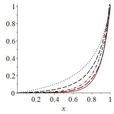
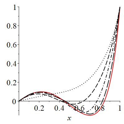
As can be seen from the graphic, step by step we can improve of the analytical solution.

1. U. Dalabaev and D. Khasanova, “An explicit expression of ordinary difference schemes for differential equations by the moved node method,” AIP Conf. Proc., vol. 3004, no. 1, p. 060043, 2024. doi: 10.1063/5.0145881.
2. G. D. Smith, Numerical Solution of Partial Differential Equations: Finite Difference Methods, 3rd ed. Oxford, UK: Oxford University Press, 1985. ISBN: 978-0198596509.
3. R. D. Richtmyer and K. W. Morton, Difference Methods for Initial-Value Problems, 2nd ed. New York, NY, USA: Wiley-Interscience, 1967. ISBN: 978-0470720400.
4. S. V. Patankar, Numerical Heat Transfer and Fluid Flow. Washington, DC, USA: Hemisphere Publishing Corporation, 1980. ISBN: 978-0070487406.
5. A. A. Samarskii, Introduction to the Theory of Difference Schemes. Moscow, Russia: Nauka, 1971. (In Russian).
6. R. E. Mickens, Nonstandard Finite Difference Models of Differential Equations. Singapore: World Scientific, 1994. ISBN: 978-9810214586.
7. R. E. Mickens, “Calculation of denominator functions for nonstandard finite difference schemes for differential equations satisfying a positivity condition,” Numer. Methods Partial Differ. Equ., vol. 23, no. 3, pp. 672–691, 2007. doi: 10.1002/num.20198.
8. R. E. Mickens, “Exact solutions to a finite-difference model of a nonlinear reaction-advection equation: Implications for numerical analysis,” J. Differ. Equ. Appl., vol. 8, no. 9, pp. 823–847, 2002. doi: 10.1080/1023619021000037086.
9. E. M. Adamu, K. C. Patidar, and R. R. Mickens, “An unconditionally stable nonstandard finite difference method to solve a mathematical model describing visceral leishmaniasis,” Math. Comput. Simul., vol. 187, pp. 171–190, 2021. doi: 10.1016/j.matcom.2021.03.006.
10. M. E. S. Begaray-Fesquet and B. B. Garay-Fesquet, “Extending nonstandard finite difference schemes rules to systems of nonlinear ODEs with constant coefficients,” Math. Numer. Anal., vol. 12, 2021.
11. A. A. Ç. Köroğlu, “Exact and nonstandard finite difference schemes for the Burgers equation B(2,2),” Turk. J. Math., vol. 45, pp. 647–660, 2021.
12. D. U. Dalabaev, “Difference analytical method of the one-dimensional convection-diffusion equation,” Int. J. Innov. Sci. Eng. Technol., vol. 3, pp. 234–239, 2016.
13. D. U. Dalabaev, “Computing technology of a method of control volume for obtaining of the approximate analytical solution to one-dimensional convection-diffusion problems,” Open Access Library J., vol. 5, p. e504962, 2018.
14. U. Dalabaev and R. Abdurakhmanov, “A simple way to solve boundary value problems in technological processes,” J. Appl. Math. Comput., vol. 23, no. 4, pp. 456–462, 2023.
15. D. U. Dalabaev and X. D. X., “The approximation error of ordinary differential equations based on the moved node method,” Probl. Comput. Appl. Math., vol. 5, no. 24, pp. 5–9, 2022.
16. D. U. Dalabaev, “Application of the method of moving nodes to solving applied boundary value problems,” Bull. Inst. Math., vol. 6, pp. 5–9, 2018.
17. R. Abdurakhmanov and D. U. Dalabaev, “Computational technology for improving the quality of difference schemes based on moving nodes,” J. Comput. Math. Appl., vol. 1860, pp. 112–118, 2021.
18. S. A. V. P. N., Numerical Methods for Resolving Convection-Diffusion Problems. Moscow, Russia: Book House “LBROKOM”, 2015.
19. S. A. A. V. B., Difference Methods for Elliptic Equations. Moscow, Russia: Nauka, 1976.
20. S. A. N. E. S., Methods for Solving Grid Equations. Moscow, Russia: Nauka, 1978.

Citations by Dimensions

Citations by PlumX

Crossref Citations

This paper is currently not cited.

No. of Downloads per Month

No. of Downloads per Country