Interior gateway protocols (IGPs) have gained popularity in networking technologies due to their capacity to enable standardized and flexible communication among these algorithms. In autonomous systems (AS), network devices communicate with one another via IGPs. This work presents a fresh investigation into the performance of inner gateway protocols in large-scale enterprise topologies. Also, the experiment lab using GNS3 simulation has been conducted to evaluate and examine the performance of RIP, EIGRP, OSPF, and IS-IS, taking into account convergence time, latency, and jitter in large-scale network topology. The work has used a tri-connected architecture, with ten (10) routers connected via three serial connections and fifteen (15) network subnets, resulting in thirty (30) different paths for routing data packets for each tested routing technique. End-to-end delay, jitter, and convergence time are three measurement measures used to investigate network topologies. The experiment’s outcomes have revealed that EIGRP has superior delay and convergence time performance. Furthermore, the results have been showed that IS-IS outperformed OSPF in terms of convergence time. Overall, this work improves the field by giving a grand average computation approach for measuring the jitter metric, which has been compared to a standard method. The method has been thoroughly explored utilizing derivate statistical equations and associated pseudo code.

1. Introduction

Interior Gateway Protocols (IGPs) are routing protocols used to exchange routing information within an autonomous system (AS), such as a corporate network or a campus network. IGPs are essential for ensuring efficient and reliable communication among the routers and hosts within an AS. However, as the size and complexity of enterprise networks increase, so do the challenges and requirements for IGPs.

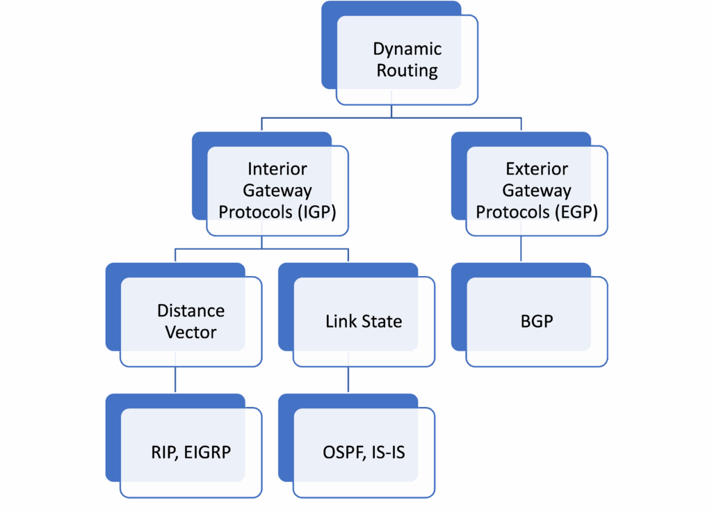
The process of routing involves determining the most efficient path for the flow of traffic within one or more networks. Routers utilize specific protocols that enable them to exchange relevant information on remote networks and update their routing tables regularly. These routing protocols determine the best path for each network, showcasing the interconnections among all routers within the network. This, in turn, facilitates communication primarily among neighboring routers and eventually throughout the entire network [1]. Routing can be classified into two categories: static and dynamic, as shown in Figure 1.

Static routing refers to the manual configuration of IP addresses and the manual entry of routes into the routing table by the network administrator before the routing process starts. Such routes can only be modified by the administrator and do not adapt to changes in the network, making them less suitable for large and unpredictable networks. They do not consume CPU memory or link bandwidth, nor do they transmit information that can be intercepted by hackers:[1]. 

In contrast, dynamic routing utilizes routing protocols that allow the network administrator to input the protocol syntax instead of manually entering each IP address. These protocols are advantageous and practical in real-time as they can detect changes within the network and determine the shortest path. They read routing update messages and adjust to changing network conditions by recalculating the shortest path and transmitting the message:[2].

This article is organized into several sections. Section 2 covers Interior Gateway Protocols, while Section 3  is about related works. Section 4 discusses the problem statement, and Section 5 presents the proposed work. Section 6 describes the network topology model and measurement methodology. Section 7 presents the experiment results and proposed mathematical equations and comparing to the basic conventional one, and section 8 presents the discussion and Section 9 concludes the overall work of this article.

2. Interior Gateway Protocols

This section provides an overview of dynamic routing protocols in local area networks: Dynamic routing protocols can be classified into three main types: distance-vector, link-state, and hybrid.   Distance-vector protocols rely on periodic exchanges of routing information between neighboring routers. Each router advertises the distance and direction to reach a destination network to its neighbors. Distance-vector protocols do not require routers to have a complete knowledge of the entire network topology. These protocols involve sending all or a portion of a router’s routing table to adjacent routers. Examples of distance-vector protocols are RIP (version 1 and 2) and IGRP. Link-state protocols, on the other hand, require routers to collect link state information from all routers in the network and construct a network map based on that information.   Then, each router calculates the best routes to each network using the network map. OSPF and IS-IS are examples of link-state protocols. Hybrid protocols combine the features of both distance-vector and link-state protocols.

2.1. RIP

Routing Information Protocol (RIP), a distance vector routing protocol, uses hops as the primary criterion for selecting a quality route. A maximum of 15 hops is allowed for RIP.   RIP is also known as the Ford-Fulkerson or Bellman-Ford algorithm. There are three main versions of RIP: RIP v1, RIP v2, and RIPng. RIP information is carried in UDP packets. The port number for RIP V1 and V2 is 520 and the port number for RIPng is 521.The administrative distance assigned to the RIP protocol is 120. Routers that use RIP send their routing tables to their neighbors every 30 seconds. The updates are sent to the multicast address 224.0.0.9 for V1 and V2. The updates for RIPng are sent to the multicast address FF02 :: 9.

2.2. EIGRP

The Enhanced Interior Gateway Routing Protocol (EIGRP) is a hybrid routing protocol that combines the features of link-state and distance-vector protocols. It uses various criteria such as delay, bandwidth, reliability, and load to select the optimal path. It employs the Diffusion Update Algorithm (DUAL) for fast convergence and effective route optimization. It also uses the Reliable Transport Protocol (RTP) for delivering EIGRP packets. There are two versions of EIGRP: EIGRPv4 for IPV4 and EIGRPv6 for IPV6. The administrative distance of EIGRP is 90 by default, with a maximum hop count of 255. It sends packets to the multicast address 224.0.0.10 and uses the port number 88. Internal routes have an administrative distance (AD) of 90, while external routes have an AD of 170. The EIGRP metrics are computed using the constants K1 = 1, K2 = 0, K3 = 1, K4 = 0, and K5 = 0, as shown in (1), and in (2):.[3]

$$\text{Metric} = \left[ K1 \times \text{bandwith} + \left( \frac{K2 \times \text{bandwith}}{256 – \text{load}} \right) + K3 \times \text{delay} \right] \times \left( \frac{K5}{\text{reliability} + K5} \right) \times 256 \tag{1}$$

$$\text{Metric} = 256 \times (\text{Bandwith} + \text{delay}) \tag{2}$$

2.3. OSPF

The Open Shortest Path First (OSPF) routing protocol utilizes Dijkstra’s algorithm, a link-state routing algorithm. Dijkstra’s algorithm calculates the shortest paths to all destinations from a source node, rather than a single source and destination pair, differing fundamentally from the Bellman-Ford algorithm and distance vector routing protocols. The routing metric in OSPF depends on the cost of a link. OSPF does not restrict the number of hops in a route. OSPF exists in two primary versions for IPv4(OSPFv2) and IPv6 (OSPFv3) networks, operating under the same principles. In OSPF, each router generates Link State Advertisements (LSAs) to establish and maintain a consistent representation of the routing topology across the entire domain. OSPF routers collect the network’s link state data and store it in a Link State Database (LSDB). Each OSPF router determines the shortest path to each network segment using the Shortest Path First (SPF) algorithm. The well-known port for OSPF is 89. OSPF uses an administrative distance of 110. OSPFv2 utilizes multicast address 224.0.0.5, while OSPFv3 uses multicast address FF02::5. The OSPF metrics are illustrated in (3) [3].

$$\text{Cost} = \frac{10^8}{\text{bandwith}} \; (\textit{bps}) \tag{3}$$

2.4. OSPF

The Intermediate System to Intermediate System (IS-IS) routing protocol operates similarly to OSPF. IS-IS is a link-state protocol developed by the International Organization for Standardization (ISO)  [4]. Like OSPF, IS-IS utilizes a link state database and Dijkstra’s Shortest Path First (SPF) algorithm to determine the shortest path routes. IS-IS supports four distinct routing metrics: default, delay, expense, and error.

IS-IS does not limit the number of hops in routes and has an administrative distance of 115. IS-IS routers can be classified as level 1, level 2, or level 1-2 routers. Level 1 routers do not have direct connections to other areas, while level 2 routers connect multiple areas, similar to OSPF Area Border Routers (ABRs). Level 1-2 routers function as both level 1 and level 2 routers, connecting their area to the backbone.

3. Related Works

This study [2] focuses on the comparison of routing protocols used in computer networks and their performance metrics, including end-to-end delay, throughput, and convergence duration. The study utilizes the Optimized Network Engineering Tool (OPNET MODELER) to simulate different network topologies and compare the performance of three routing protocols: RIP, EIGRP, and OSPF. The simulation results show that OSPF has the fastest throughput among the three protocols, while EIGRP has the fastest convergence time. Additionally, EIGRP has faster throughput than RIP, but RIP has the highest queuing delay. This study provides valuable insights into the performance of different routing protocols and their suitability for different network topologies, but the methods of calculating performance metrics were not clarified, and the Riverbed Modeler they relied upon.

This study [5] compares the performance of EIGRP and OSPF routing protocols in terms of convergence time with link failures and the addition of new links in different network scenarios. The research uses a network simulator called GNS3 to simulate network topologies and validates the results using Cisco hardware equipment in the laboratory. The study finds that EIGRP has a faster convergence time than OSPF with a link failure or a new link added to the network. The experiment contributes to existing knowledge by identifying that the mesh topology has the best convergence time and that hardware implementations of routing protocols are better than using a network simulator. The study recommends further research in comparing BGP with EIGRP and OSPF and analyzing the protocol changes or adaptations in terms of convergence time with the versions of IPV4 and IPV6. Additionally, latency and quality of service are identified as vital areas of research in both EIGRP and OSPF routing protocols. The Wireshark results are used to check the network configuration and monitor accurate time responses for the various packets.

This study [6] compares the performance of two routing protocols, RIPv2 and EIGRP, in terms of data packet routing speed and convergence time. The research uses the Cisco Packet Tracer 7.10 software to simulate full mesh and half mesh topologies and conducts various tests, such as network connectivity, traceroute, and time testing. The study finds that EIGRP has a faster convergence time and routing speed than RIPv2 in both topologies. The results of the analysis suggest that EIGRP’s hybrid routing characteristics (distance vector and link state) enable faster selection of vector-based paths and that EIGRP updates only the routing table of affected routers, while RIPv2 updates the routing table of all routers. The study concludes that EIGRP is a better routing protocol for an institution or college network that requires proper and safe network methods.

This study [7] aims to assess and compare the performance of different interior gateway routing protocols in an enterprise-level network that is complicated and operates in real-time. This is achieved by utilizing the GNS3 software to simulate the network, which consists of hosts, switches, and routers, and by putting each protocol into the topology. The protocols that have been examined are EIGRP, OSPF, and RIP. The authors guarantee secure data transmission at each node by offering authentication, and the assessment criteria include throughput, end-to-end delay, and convergence time. The study’s findings indicate that EIGRP is the most practicable interior gateway routing protocol for a complicated enterprise-level network since it performs the best in terms of convergence time. In stable network conditions, there are no major differences observed in the end-to-end delay and throughput values of the three protocols; OSPF has a higher throughput than RIP and less significant delays than both RIP and EIGRP.

This study [8] aims to assess and contrast the effectiveness of many Interior Gateway Routing Protocols (IGRPs), more especially OSPF, RIPV2, and EIGRP. Using Graphical Network Simulator (GNS-3) simulations, the authors analyzed a number of characteristics, including throughput, jitter, convergence time, end-to-end delay, and packet depletion. EIGRP performs better than OSPF, according to the results. It was also mentioned that EIGRP uses greater processing power, which increases the system’s power usage.

This study [6] the convergence times of the EIGRP and RIPv2 routing protocols were compared by the authors. Cisco Packet Tracer 7.10 was used to run the simulation on two different network topologies: full mesh and half mesh. The findings showed that the RIPv2 protocol took longer to converge—ranging from 0.01 to 0.19 seconds—while the EIGRP protocol had a faster average convergence time of 0.01-0.02 seconds.

4. Problem Statement

Network hardware performance is influenced by several factors, including convergence, delay, and jitter. Achieving optimal performance requires selecting the appropriate combination of routing protocols. Despite extensive research on interior gateway protocols, detailed computation of convergence, delay, and jitter has not been sufficiently addressed in these studies. In contrast, our paper employs equations to calculate these factors, providing a more comprehensive and accurate evaluation of network hardware performance, then the proposed analysis has .

5. Proposed Work

The primary aim of this work is to evaluate and analyze the performance of a complex enterprise network by considering convergence, delay, and jitter, and utilizing Interior Gateway Protocols such as OSPF, EIGRP, and IS-IS. Furthermore, the study seeks to determine the most suitable protocol for large-enterprise topologies. Notably, this research contributes to the field by introducing an enhancement analysis of the “delay, jitter, which is a factor in achieving optimal network performance. In order to obtain a higher accuracy measured value than the fundamental traditional method, the grand average statistical method has been utilized in the proposed method to quantify jitter, “delay”, in a large-scale network topology. In order to determine the differences in the jitter, “delay”, in the proposed Tri-connected network devices topology in this work, a comparison is made between the suggested approach and the conventional one using the interior gateway routing protocols.

6. Models and Measurement Parameters

This section provides an overview of the devices and media types employed in setting up the network topology, as well as an examination of the software used. Additionally, the measurement parameters used to analyze the network topologies are described.

Partial mesh (Tri-connected) topology is a network topology combining features of full mesh and star topologies, providing high fault tolerance and redundancy. It is commonly used in medium to large enterprises, offering a scalable traffic handling capability. Nodes are connected to a subset of other nodes or all nodes in the network. It is ideal for medium to large enterprises requiring a network that can handle a moderate to a high amount of traffic. Partial mesh topology is less expensive than a full mesh topology. It is an effective solution for enterprise networks that require fault tolerance, redundancy, and scalability.

The proposed network topologies comprise ten routers interconnected through three serial connections, with 15 network subnets forming 30 multiple paths for routing data packets for each assessed routing protocol. This configuration results in a complex network topology at the enterprise level, as illustrated in Figure 2 below.

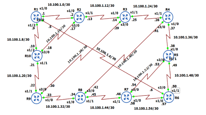
The proposed large-scale infrastructure is built to ensure it ideal for enterprise applications and the complexity of network devices. The network configuration is built to meet the following:

1. Network topology: ten (10) routers connected via three (3) serial connections to interconnect using a single channel to routing packets.
2. Subnets: fifteen (15) different subnets to ensure the complexity of the topology.
3. Routing path: thirty ( 30) routing path for data packet routing (Tri-connected 10 routers).
4. Routing protocol: various interior routing protocols assessed for efficiency.
5. Network topology Size: Large-scale network topology

6.1. Hardware and software resources

This subsection provides details on the hardware and software resources utilized for the simulation and testing. The IP addressing configuration and network topology used in the experiments are illustrated in Figure 2 above. The network topology comprises ten Cisco 7200 routers, providing multiple paths between different sections of the topology. The routers used in the experiments are identical in model and specifications, as listed in Table 1. The software used to perform the experiments is GNS3 version 2.2.34, while the HP ProBook 450 5G was used as the testing device, with its specifications outlined in Table 2.

Table 1: Network devices employed in the network topology

Table 2: Laptop device specification for Personal Computer use.

From the standpoint of three initial parameters, network performance was examined using the same network topology and different protocols.

The measurement parameters would be used in this work can be defined as follows:

A) End to end delay

The total time required for a complete message to travel from its source to destination encompasses the duration from the initial transmission of the first bit of the message until the final delivery of the last bit of the message.

B) Jitter

The variation in packet delay, commonly referred to as packet delay variance, is an indication of the presence of jitter when data packets experience disparate delays across a network. Jitter is often measured in milliseconds (MS).

C) Convergence time

The metric measures the speed at which a group of routers restores a network to its normal state.

7. Experiment Results

In this section, each interior gateway protocol presented in this paper was evaluated to determine the most suitable protocol for the network topology under consideration. This evaluation was based on the calculation of end-to-end delay, convergence time, and jitter, in accordance with the study’s objectives.

7.1. End-to-End Delay Testing Results

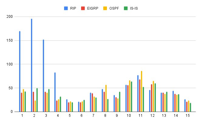
Table 3 presents the average end-to-end delay values for EIGRP, OSPF, and IS-IS, which were determined using the ping utility throughout the analysis.

Table 3: The average end-to-end delay values for the RIP, EIGRP, OSPF, and IS-IS protocols calculated for each subnet

Table 3 represents end to end delay for each protocol by taking the average of round-trip time (RTT) by using ping utility. Figures. 3, 4, and 5 represent samples of results of sixty (60) experiments for four (4) measured interior gateway routing protocol for fifteen (15) different subnets.

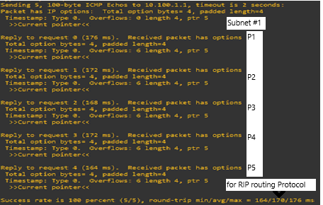
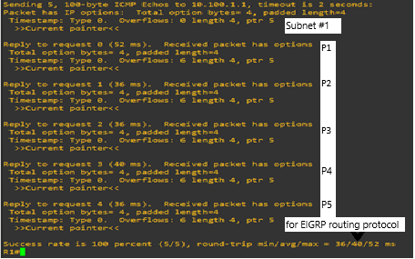
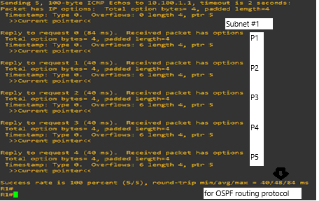
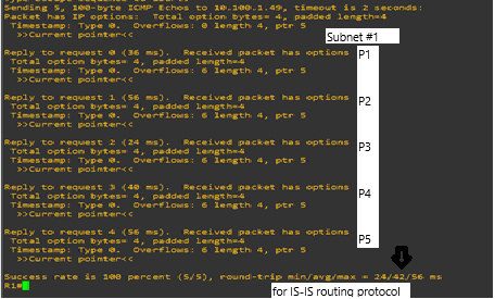
The obtained results of the previous four Figures are measured using Ping utility using Internet Communication Message Protocol (ICMP) echoes. The round-trip is measured through packet traveling using different interior  gateway routing protocol in each time using the same large-scale proposed network topology. As shown above, the results are different from one interior gateway routing protocol to other interior gateway routing protocol.

Figure 7 represents the delay variation, from the values in Table 3, so can see that for the 1st case EIGRP has the least delay, whereas the 2nd and the 3rd case OSPF has the least delay. For the 4th, 5th and 6th case EIGRP has the least delay. For the 7th and 8th  case IS-IS has the least delay. For the 9th ,13th and 14th OSPF has the least value. So EIGRP has the least delay among the OSPF and IS-IS.

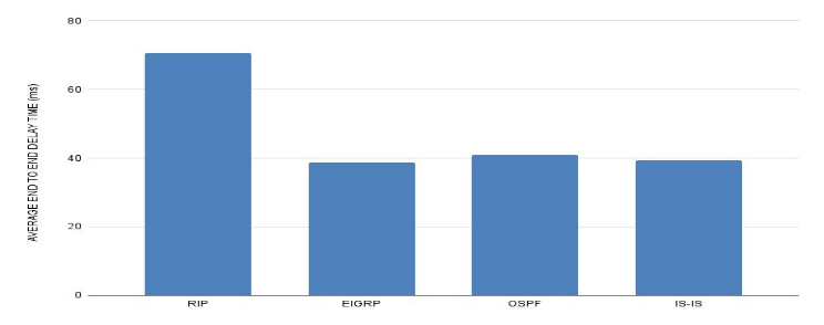
The Table 4 below displays the average values of the end-to-end delay for RIP, EIGRP, OSPF, and IS-IS which has been computed by taking the average of the Table 3 averages for each protocol separately.

Table 4: Comparison of Average End to End Delay for RIP, EIGRP, OSPF and IS-IS.

The Figure 8 below represents the average end-to-end delay from the values in Table 4, and by analyzing Figure. 7, can see that EIGRP has the least average value of delay and does not differ much from IS-IS and OSPF. Figure 7 shows that OSPF has the worst average value of delay. 

7.2. In depth analysis for Jitter Testing Results

A) Proposed Method

In this section, to obtain the most accurate jitter result, a delay of 75 packets (fifteen (15) subnets multiplied by five (5) received messages using Ping utility using ICMP echoes) has been calculated for each protocol, and 60 jitter results were obtained for all interior gateway routing protocol By calculating the differences between the delays for the five packets, respectively, as shown in Tables 5, 6, 7, and 8 below.

An example of this is that the result of the first jitter is the difference between the delay for the first and second packets, and the result of the second jitter is the difference between the delay for the second and third packets, and so on. Let R represents the jitter result, i represents the number of received packet sequence within one subnet, and P represents packet delay as shown in (4).

$$R_i = \left| P_{i+1} – P_i \right| \tag{4}$$

The Table 9 below displays the average values of the in-depth analysis of jitter for RIP, EIGRP, OSPF, and IS-IS, which has been calculated by taking the average of 60 (the volume of the data packets is equal to fifteen (15) subnets multiply by four (4) different interior gateway routing protocols) values of jitter from the Tables 5, 6, 7, and 8 above for each protocol separately. Let R represent the Jitter result for each two send packets obtained in (4), i represent the iteration of measurement jitters in each subnet, and K represents the number of jitter results equal to 4 (i-th of 4) for each interior gateway routing protocol, and AVG is the average value of jitter measure calculated in each subnet iteration (i-th of 15).

$$AVG_{ith} = \frac{\sum_{i=1}^{K} R_i}{K} \tag{5}$$

Table 5: In depth analysis JITTER result for RIP.

Table 6: In depth analysis JITTER result for EIGRP

Table 7:  In depth analysis JITTER result for OSPF

Table 8:  In depth analysis JITTER result for IS-IS

In order to get the grand average (GAVG) of each jitter measured interior routing protocol in the proposed network topology that has fifteen (15) subnets the calculation in (6) has been used, using the obtained measured of average iteration values in (5) for each subnet (S of total of fifteen (15) in this experiment).

$$GAVG = \frac{\sum_{ith=1}^{S} AVG_{ith}}{S} \tag{6}$$

The Table 9 shows the calculated grand average of overall measured value for jitter in the proposed large-scale enterprise network topology, refer to Figure 2 above. These measured values are obtained using the proposed method that is presented in this work.

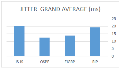
Table 9: Comparison of Average jitter for RIP, OSPF, EIGRP and IS-IS using proposed method

The Figure 9 below represents the grand average jitter from the values in Table IX, OSPF’s routing protocol has the lowest average value of jitter compared to RIP protocols, EIGRP protocol, and IS-IS protocol. Especially IS-IS, the IS-IS protocol has the highest average value of jitter.

B) Traditional Method to measure Jitter

This section also presents the classic technique of calculating Jitter, which is a well-known method for calculating the variance of only the first and second packets of replay to the requests messages using ICMP Echoes: [9], [10], [11] and [12].

Table 10 shows the calculated grand average of overall measured values for jitter in the proposed large-scale enterprise network topology, refer to Figure 2. These measured values are obtained using the traditional method of jitter metric, refer to Tables 5, 6, 7, and 8 above for each protocol separately.

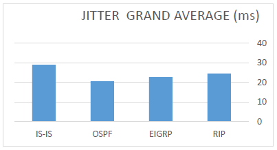
Table 10: Comparison of Average jitter for RIP, OSPF, EIGRP and IS-IS using traditional method

The Figure 10 below represents the grand average jitter from the values in Table 10, OSPF’s routing protocol has the lowest average value of jitter compared to RIP protocols, EIGRP protocol, and IS-IS protocol. Especially IS-IS, the IS-IS protocol has the highest average value of jitter.

In order to get more clear of the results of both traditional mothed and proposed method, the comparing are shown in Figure 11 and in Table 11. The variance between both method is clear and indicate the difference that should be taken in account when measuring the Jitter metric especially in the large-scale enterprise network topology.

Table 11: Comparison of grand Average jitter for RIP, OSPF, EIGRP and IS-IS using traditional and proposed methods.

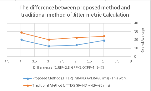
The Figure 11 above shows the differences that should be considered to pick the accuracy method to measure the Jitter in small, mid-sized, or large-scale network topology. The new method uses in-depth analysis technique using statistical method to improve the result of the measure using all reply messages to calculate the grand average when compare it to the traditional measuring method. The pseudo code for Jitter calculation using the proposed method in this work is illustrated program algorithm 1 below:

7.3. Convergence Time Testing Results

When a route becomes unavailable, the router requires a certain amount of time to notify other routers of the failure and determine the best alternative path [13], [14], [15] and [16].

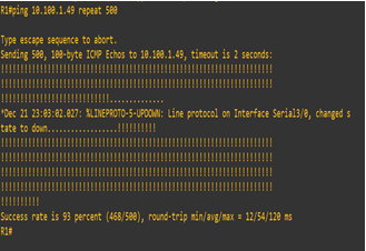
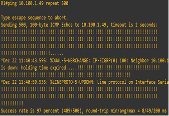
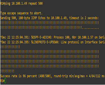
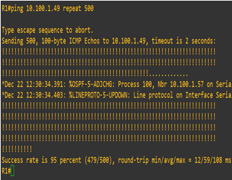
This process is commonly referred to as the convergence of time. In our experiment, packets of 100-datagram size and a 2-second timeout were transmitted from the source to the destination with a repeat count of 500. While sending these packets, we intentionally disrupted one of the routes and observed the subsequent loss of packets until the new path information was fully propagated to all routers. To determine the convergence time, we calculated the number of lost packets and multiplied it by the 2-second timeout. This process was repeated five times, and the average was calculated. Refer to Figures 12, 13, and 14 below.

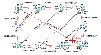
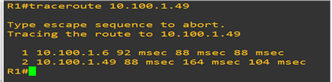
Table 12: Convergence Time of RIP.

Table 13: Convergence Time of EIGRP

Table 14: Convergence time of ospf

Table 15: Convergence Time of IS-IS.

Tables 12, 13, 14, and 15 above represent the convergence times and the average convergence times for each protocol. Figures 15, 16, 17, and 18 below represent samples of results.

The Figure 19 below represents the average of convergence time from the values in Tables 12, 13, 14, and 15 above, and by analyzing Figure 19, so can see that EIGRP has the least average value of convergence time and the OSPF has the worst average value of convergence time.

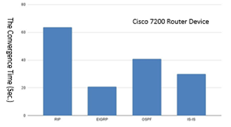
As explained in the beginning of the sub-section “7.3”, conversion time is calculated after the failure of one or more network router device in the network topology and the least measured value is the best recoverable protocol. The obtained result from the experiment indicate that the EIGP is more suitable for large-scale enterprise network topology.

8. Discussion

Many research papers have been presented the evaluation of the interior gateway routing protocols in different network topologies, each topology has different characteristics like the number of routing paths that used in their experiments, number of network devices, topology type as small; mid-sized; or large-scale network, number of subnets used in their experiments, internet protocol versions that used, default cost variation, route table size, dropped traffic and so on:[16][17][18] and [19].

Also there are different techniques have been used to measure the metric of these interior gateway routing protocols regardless of the network topology especially when measure the jitter to evaluate the performance of the network: [12] [19] and [20]. Here, in this work, the evaluation of these interior gateway protocols has been conducted in a large-scale network topology consist of 30-routers with tri-connected interfaces. A new method to calculate the Jitter has been presented in detail with its pseudo code and then compared with the simple technique method of measuring the Jitter in the computer networks. The result has shown there is a big different in term of the accuracy of both calculation methods, but both the jitter measurement methods have the same curve pattern.

9. Conclusion

This study compared the performance of RIP, EIGRP, OSPF, and IS-IS inner gateway protocols in terms of convergence time, end-to-end delay, and jitter for fifteen subnets in proposed network topologies. The results show that EIGRP outperformed other routing protocols in terms of latency and convergence time, although OSPF outperformed them in terms of jitter. In addition, IS-IS outperformed OSPF in terms of convergence time. In contrast, the results showed that RIP protocols had the poorest delay and convergence time performance. Finally in this work, it has introduced a new method for measuring jitter. The formula was developed to calculate network jitter with greater accuracy than the traditional, convention, method using the grand average calculations. Additionally, the suggested method may be replicated to model various network topology sizes, and the new approach can be contrasted with other methods to improve the speed and precision of jitter measurement in the field of routing networks. This would develop and improve new monitoring tools to measure jitter networks more accurately and quickly.

Conflict of Interest

The authors declare no conflict of interest.

1. M. Usman, E.E. Oberafo, M.A. Abubakar, T. Aminu, A. Modibbo, S. Thomas, “Review of interior gateway routing protocols,” in 2019 15th International Conference on Electronics, Computer and Computation, ICECCO 2019, 2019, doi:10.1109/ICECCO48375.2019.9043204.
2. (PDF) Performance Comparison of Routing Protocols | yousef aburawi – Academia.edu, Oct. 2024.
3. A.G. Biradar, “A Comparative Study on Routing Protocols: RIP, OSPF and EIGRP and Their Analysis Using GNS-3,” 2020 5th IEEE International Conference on Recent Advances and Innovations in Engineering, ICRAIE 2020 – Proceeding, 2020, doi:10.1109/ICRAIE51050.2020.9358327.
4. C. Filsfils, A. Bashandy, H. Gredler, B. Decraene, “IS-IS Extensions for Segment Routing,” 2019, doi:10.17487/RFC8667.
5. I. Joseph Okonkwo, I. Douglas Emmanuel, “Comparative Study of EIGRP and OSPF Protocols based on Network Convergence,” IJACSA) International Journal of Advanced Computer Science and Applications, vol. 11, no. 6, 2020.
6. D.R. Prehanto, A.D. Indriyanti, G.S. Permadi, “Performance analysis routing protocol between RIPv2 and EIGRP with termination test on full mesh topology,” Indonesian Journal of Electrical Engineering and Computer Science, vol. 23, no. 1, 354–361, 2021, doi:10.11591/IJEECS.V23.I1.PP354-361.
7. M. Athira, L. Abrahami, R.G. Sangeetha, “Study on network performance of interior gateway protocols — RIP, EIGRP and OSPF,” 2017 International Conference on Nextgen Electronic Technologies: Silicon to Software (ICNETS2), 344–348, 2017, doi:10.1109/ICNETS2.2017.8067958.
8. A. Manzoor, M. Hussain, S. Mehrban, “Performance Analysis and Route Optimization: Redistribution between EIGRP, OSPF & BGP Routing Protocols,” Computer Standards & Interfaces, vol. 68, 103391, 2020, doi:10.1016/J.CSI.2019.103391.
9. (PDF) Performance Analysis of Interior Gateway Protocols, https://www.researchgate.net/publication/303812574_Performance_Analysis_of_Interior_Gateway_Protocols, Oct. 2024.
10. H. Karna, V. Baggan, A.K. Sahoo, P.K. Sarangi, “Performance Analysis of Interior Gateway Protocols (IGPs) using GNS-3,” Proceedings of the 2019 8th International Conference on System Modeling and Advancement in Research Trends, SMART 2019, 204–209, 2020, doi:10.1109/SMART46866.2019.9117308.
11. What Is Jitter, and How Does It Affect Your Internet Connection?, https://www.howtogeek.com/824032/what-is-jitter/, Oct. 2024.
12. How to Measure Jitter – Obkio, https://obkio.com/blog/how-to-measure-jitter/, Oct. 2024.
13. IMPROVING THE PERFORMANCE OF AD HOC NETWORK USING ENHANCED INTERIOR GATEWAY ROUTING TECHNIQUE – IJSER Journal Publication, https://www.ijser.org/onlineResearchPaperViewer.aspx IMPROVING_THE_PERFORMANCE_OF_AD_HOC_NETWORK_USING_ENHANCED_INTERIOR_GATEWAY_ROUTING_TECHNIQUE.pdf, Oct. 2024.
14. N. Kumari, D.T. Raj, “OSPF Metric Convergence and Variation Analysis During Redistribution with Routing Information Protocol,” International Research Journal on Advanced Engineering and Management (IRJAEM), vol. 2, no. 06, 1985–1991, 2024, doi:10.47392/IRJAEM.2024.0293.
15. E.C. Obioma, E.C. Amadi, “Analysis of Optimal Routing Protocol for an Inter-Campus Private Cloud Network System,” International Journal of Modern Developments in Engineering and Science, vol. 3, no. 2, 8–12, 2024, doi:10.5281/ZENODO.12643596.
16. K. Shahid, S.N. Ahmad, S.T.H. Rizvi, “Optimizing Network Performance: A Comparative Analysis of EIGRP, OSPF, and BGP in IPv6-Based Load-Sharing and Link-Failover Systems,” Future Internet, vol. 16, no. 9, 2024, doi:10.3390/FI16090339.
17. N. Kumari, A. Sharma, “OSPF Default Cost Variation for Type-1 and Type-2 External Links during Redistribution,” International Journal of Computer Applications, vol. 184, no. 28, 8–14, 2022, doi:10.5120/IJCA2022922345.
18. M.E. Mustafa, ; Ahmed, A. Abaker, “International Journal of Computer Science and Mobile Computing Evaluate OSPF and EIGRP Based on Route Table Size and Dropped Traffic using Different Topologies (Star, Loop),” International Journal of Computer Science and Mobile Computing, vol. 13, 6–17, 2024, doi:10.47760/ijcsmc.2024.v13i04.002.
19. D. Turlykozhayeva, S. Temesheva, N. Ussipov, A. Bolysbay, A. Akhmetali, S. Akhtanov, X. Tang, “Experimental Performance Comparison of Proactive Routing Protocols in Wireless Mesh Network Using Raspberry Pi 4,” Telecom 2024, Vol. 5, Pages 1008-1020, vol. 5, no. 4, 1008–1020, 2024, doi:10.3390/TELECOM5040051.
20. Performance Analysis of Routing Protocols RIP, EIGRP, OSPF and IGRP using Networks connector, 2020, doi:10.4108/eai.28-6-2020.2298167.

Citations by Dimensions

Citations by PlumX

Crossref Citations

This paper is currently not cited.

No. of Downloads per Month

No. of Downloads per Country