
Edge-AI Fusion of Downhole IoT Sensor Streams for Real-Time Kick Detection in High-Pressure High-Temperature Wells: A Synthetic-Simulator Feasibility Study

(This article belongs to the Section Petroleum Engineering (PTE))
Export Citations
Cite
Khose, V. (2026). Edge-AI Fusion of Downhole IoT Sensor Streams for Real-Time Kick Detection in High-Pressure High-Temperature Wells: A Synthetic-Simulator Feasibility Study. Journal of Engineering Research and Sciences, 5(11), 26–37. https://doi.org/10.55708/js0511002
Vishal Khose. "Edge-AI Fusion of Downhole IoT Sensor Streams for Real-Time Kick Detection in High-Pressure High-Temperature Wells: A Synthetic-Simulator Feasibility Study." Journal of Engineering Research and Sciences 5, no. 11 (November 2026): 26–37. https://doi.org/10.55708/js0511002
V. Khose, "Edge-AI Fusion of Downhole IoT Sensor Streams for Real-Time Kick Detection in High-Pressure High-Temperature Wells: A Synthetic-Simulator Feasibility Study," Journal of Engineering Research and Sciences, vol. 5, no. 11, pp. 26–37, Nov. 2026, doi: 10.55708/js0511002.
A kick, an uncontrolled influx of formation fluid, is among the most dangerous events in high-pressure high-temperature (HPHT) drilling. Surface delta-flow and pit-gain alarms are still the industry default, but they detect late and raise many false alarms. This paper asks a narrow question. Would a detector that fuses downhole Internet of Things (IoT) streams with surface data, and runs at the rig floor instead of in the cloud, find kicks sooner at a lower false-alarm rate? Labelled field kicks are not public, so we built an open Python simulator and tested on that. The proposed architecture has several parts, but only one is evaluated here, a feed-forward multi-modal fusion network (MMFNN) on seven channels. The transformer variant, the physics-informed loss, uncertainty gating, transfer learning and embedded deployment remain design. Over five independent replicates (1,250 test scenarios, 185 kicks), the MMFNN reached a mean precision of 0.97 and 0.8 false alarms per 24 h, with a median time to detect of 24 s. A delta-flow rule in the spirit of API RP 59 gave 0.55, 20 and 45 s. Without the downhole channels the network produced 12 false alarms per 24 h and needed 46 s, and the acoustic channel accounted for most of the gain. Doubling the noise on every channel cost the MMFNN some precision and erased its small lead over a gradient-boosted model, while noise on the pressure channel alone changed nothing. Output probabilities were well calibrated overall but mildly over-confident in the middle range. A cloud-hosted variant with a 3 s round trip added that delay. Because everything is simulated, the results show feasibility, not field performance. Real-well data, embedded benchmarks and tests of the design elements are the next steps.
1. Introduction
A kick is the thing drillers fear most: formation fluid enters the wellbore faster than the mud system can hold it back. Caught early, it is a routine shut-in. Caught late, it can become a blowout. In high-pressure high-temperature (HPHT) wells, usually taken as bottom-hole conditions above 69 MPa (10,000 psi) and 150 °C, the margin between pore pressure and fracture gradient can fall below 60 kg/m³ (0.5 lb/gal), so an influx has very little room to hide. Oil-based muds make the problem worse, because gas dissolves in the mud and often shows itself only close to surface [1]. Macondo, in 2010, is still the reference case. Eleven people died, and the total cost ran into tens of billions of U.S. dollars [2].
Most rigs still depend on surface instruments. Flow paddles, pit-level sensors and standpipe pressure feed a threshold rule or a mud logger, in line with API RP 59 [3] and standard well-control practice [4]. Two things limit that approach. The first is physical. Surface flow and pit volume respond to the volume an influx displaces, not to the influx itself arriving at surface, and a small, compressible or dissolved influx displaces very little until it is well up the annulus [5]. The second is practical. Connections, pump changes and fluid losses move the same signals, so an alarm tuned for sensitivity fires on non-events. Machine learning can help, but most published detectors assume centralised inference [6, 7]. A remote rig cannot always rely on a link good enough to keep that inside the alarm path.
This paper looks at a different operating point: edge-resident detection that fuses downhole Internet of Things (IoT) streams with surface data at the rig floor. It is a feasibility study on a simulator. It does not claim field validation, and it does not test the whole architecture we describe. Only one detector is trained and scored, a feed-forward network on seven channels. Everything else is design, and Table 1 says so item by item. The contributions are:
- An open Python simulator that produces 1 Hz scenarios of nominal drilling, pump connections, lost circulation, and gas, water and oil kicks, with the governing relations written out (Section 5.1).
- A multi-modal fusion feed-forward network (MMFNN) on seven channels, compared with four baselines and a cloud-hosted variant that adds a configurable round-trip delay.
- An evaluation over five independent simulator replicates (1,250 held-out scenarios), with calibration metrics, channel ablations, and sensitivity to sensor noise, alarm threshold and network latency.
- A design description of the remaining architecture, marked as untested, with the physics residuals written out in the appendix.
Section 2 reviews related work and Section 3 formalises the detection problem. Section 4 describes the architecture and what has been tested, Section 5 the simulator and experimental protocol, and Section 6 the results. Section 7 covers limitations and Section 8 concludes.
2. Related Work
2.1. Kick Detection in Drilling Operations
Kick-detection research goes back more than six decades. It starts with the delta-flow method [3], then moves through model-based observers and pattern recognition to deep learning. The classical rules are simple and transparent. They also trip on connections, pump transients and lost circulation. A review of supervised learning for hazardous drilling events [6] shows how quickly the data-driven literature has grown. In [7], the authors built a Bayesian network over surface indicators and reported earlier warnings than conventional delta-flow alarms. In [8], they raised kick-warning sensitivity by classifying the current drilling activity first. In [9], the authors compared random forest, support vector machine, feed-forward and LSTM detectors on logging data; the best configuration responded in under two seconds. A 2026 review [10] surveys multi-source data fusion for deepwater gas kicks and links sensor observability to well-control actions. Not one of these works fuses downhole IoT streams at the rig-floor edge. That is the gap here.
2.2. Downhole Sensing and Fibre-Optic Monitoring
Distributed temperature and acoustic sensing resolve wellbore conditions at metre scale along kilometres of fibre [11]. Pressure-while-drilling (PWD) and logging-while-drilling (LWD) tools send high-rate data through wired drill pipe, but mud-pulse telemetry, still the workhorse on most rigs, carries at best tens of bits per second [12]. These streams already support flow assurance, fracture monitoring and reservoir characterisation. Their use for kick detection is still thin.
2.3. Edge Machine Learning and Industrial IoT
Edge inference is now the default for latency- and bandwidth-limited industrial work. Quantisation and runtimes such as TensorRT and ONNX Runtime make sub-100-millisecond pipelines practical on ruggedised hardware. Oil-and-gas deployments so far have mostly put edge analytics on equipment health. Well control has stayed a cloud or on-premise workflow.
2.4. Simulators and Benchmarks for Well-Control Research
Commercial simulators such as OLGA, Drillbench and LedaFlow are the accepted references for multiphase flow and dynamic drilling. They are proprietary, which limits reproducibility and makes direct comparison between research groups hard. Public field data such as the Volve release (open dataset published by Equinor in 2018) rarely contain labelled kicks, and a drilling dataset released for formation-pressure prediction and kick detection [13] is only starting to close that gap. We use a deliberately simple, open simulator for controlled comparison, and we treat cross-checks against OLGA or Drillbench, and against real wells, as required follow-on work.
3. Problem Formulation
Let Xt = {xPWD, xDTS, xDAS, xflow in, xflow out, xpit, xSPP} be the channels available at time t. At every sample the detector outputs a kick probability pt = P(kick | Xt−W:t) over a sliding window of W seconds (W = 60 in the experiments). An alarm fires when the probability stays at or above a threshold τp for m consecutive samples,
and 0 otherwise, with τp = 0.5 and m = 3 for every learned detector. The design adds a second condition, an epistemic uncertainty σt below a bound τσ; it is not used in the experiments. Time to detect for a scenario with onset t0 is
capped at 300 s when no alarm fires. The false-alarm rate counts non-kick scenarios that raise at least one alarm, normalised to 24 h of non-kick drilling,
where NFA is the number of such scenarios and Hnon-kick their total duration in hours. Three design targets frame the work. Processing latency, from a new sample to an alarm decision, should stay under one second on the target platform. The false-alarm rate should be as low as practical. Adapting to a new rig should need no more than about ten labelled real kicks. The last target is not tested here, and the first only on a proxy.
4. Proposed Method
4.1. System Architecture
The architecture has three tiers (Figure 1). A downhole sub carries a small anomaly screener on an ARM Cortex-class microcontroller, a 1-D convolutional network that watches pressure and acoustic envelopes and gates what is sent uphole. The middle tier is a rig-floor gateway, for example an NVIDIA Jetson Orin NX in a Zone-1 enclosure. It runs the fusion model, the physics checks and the explanation layer. The top tier is a cloud platform aligned with the OSDU data model, used for historian storage, cross-rig learning and reporting. By design the cloud stays out of the alarm decision path.
4.2. Multi-Modal Temporal Fusion Transformer (Design)
Each sensor modality first passes through its own stem, which normalises units, resamples to a common grid and projects into a shared embedding. A cross-modal attention block aligns the embeddings, and a temporal self-attention stack integrates a 60 s window, following the temporal fusion transformer [14]. A Bayesian head returns a kick probability and a Monte-Carlo-dropout estimate of epistemic uncertainty [15]. This model is not implemented in the present study.
4.3. Feed-Forward Fusion Network
To keep the study runnable on commodity hardware, the evaluated detector is a feed-forward stand-in for the transformer, the MMFNN. It keeps early cross-channel fusion but replaces attention with a small multilayer perceptron fed by five rolling statistics per channel over the last 60 s: current value, mean, standard deviation, delta from the window start, and end-to-end slope. With seven channels that gives 35 inputs. The hidden layers have 64, 32 and 16 units, and the output is a logistic kick probability. Figure 2 contrasts this path with the transformer design.
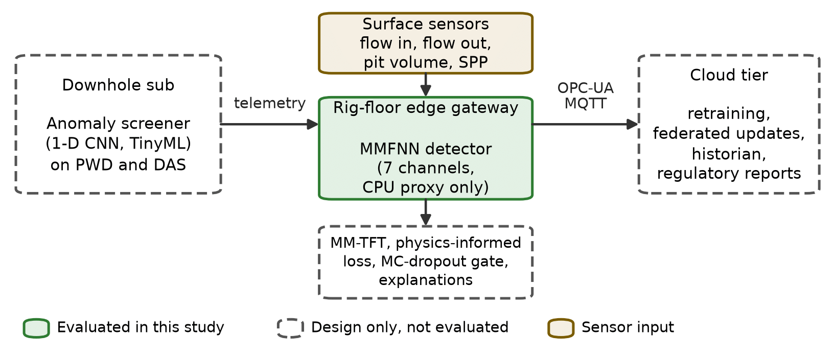
Figure 1: Three-tier edge-AI architecture. Solid green marks the part evaluated in this study (the MMFNN on the gateway, run here on a workstation CPU). Dashed outlines are design elements that were not evaluated. Beige marks sensor input. PWD: pressure while drilling; DAS: distributed acoustic sensing; SPP: standpipe pressure; MM-TFT: multi-modal temporal fusion transformer; MC-dropout: Monte-Carlo dropout; OPC-UA and MQTT: industrial messaging protocols.
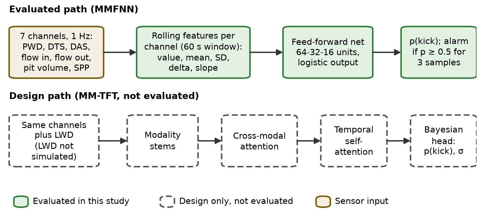
Figure 2: Evaluated and design-level model paths. The upper row is the MMFNN that was trained and scored. The lower row is the transformer design that was not implemented; it would also take LWD input, which the simulator does not generate. SD: standard deviation; delta: change from the start of the 60 s window; slope: end-to-end rate of change over the window; σ: epistemic uncertainty; LWD: logging while drilling.
4.4. Physics-Informed Loss (Design)
The design objective adds two physics terms to a weighted cross-entropy: a mud mass-balance residual built from inflow, outflow and pit-volume changes, and an equivalent-circulating-density (ECD) residual built from pressure-while-drilling readings and a hydraulics estimate. Appendix A gives both in full. None of this is in the trained model. Section 6.7 reports a lighter proxy, mass-balance features fed to the same network, and that proxy should not be read as the loss.
4.5. Edge Inference Pipeline
On the target gateway the trained model would be exported to ONNX, quantised to INT8 with per-channel calibration and compiled with TensorRT. A service would read OPC-UA and MQTT streams, expose a WebSocket interface to the driller’s display, and write signed decisions to a local historian. None of that is built. The experiments here run scikit-learn on a workstation instead, so the latency numbers are a proxy. Figure 3 shows the two-stage flow in which the downhole screener wakes the fusion model.
4.6. Transfer Learning from Simulated to Real Wells (Design)
The intended protocol pre-trains on a large simulated corpus and fine-tunes on real wells with a domain-adversarial network [16]. No real-well data were available, so the step is a design element only. The experiments below train and test on the same simulator. They are an in-distribution result, and an optimistic one.
4.7. Uncertainty Gating and Explainability (Design)
At design time an alarm needs both a high probability and a low uncertainty. Shapley attributions [17] would then be mapped to the kick indicators drillers already use [5]. The evaluated MMFNN has neither: it thresholds the probability directly. Section 6.4 checks how well that probability is calibrated.
4.8. What Has and Has Not Been Validated
A fair question is how much of the architecture the experiments touch. Table 1 answers that component by component.
5. Experimental Setup
5.1. Synthetic Kick Simulator
Every experiment runs on an in-house Python simulator released with the paper. It writes seven channels at 1 Hz over ten-minute windows. Bottom-hole pressure comes from the PWD tool, a reference-depth temperature from distributed temperature sensing (DTS), and an acoustic-energy proxy from DAS. The rest are flow in, flow out, active pit volume and standpipe pressure (SPP). The nominal operating point is 2,461 L/min (650 gpm) of flow, 82.7 MPa (12,000 psi) at the bit, 165 °C, 79.5 m³ (500 bbl) in the active pits and 24.1 MPa (3,500 psi) at the standpipe. Each channel gets Gaussian noise and a slow drift made of a random walk plus a one-cycle sinusoid. Zero to two short pump surges per window add 38 to 95 L/min (10 to 25 gpm) to flow out. They give the surface rules something to trip on.
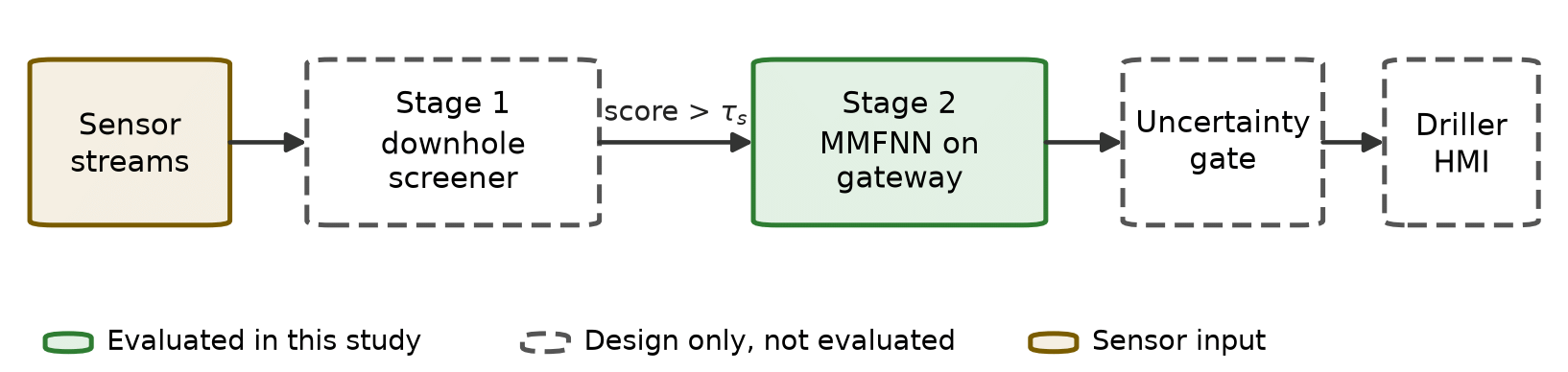
Figure 3: Two-stage edge inference pipeline. Stage 1 runs downhole and forwards data when its anomaly score exceeds a threshold τs. Stage 2 is the fusion model on the rig-floor gateway. Only Stage 2 (MMFNN) was evaluated. HMI: human-machine interface.
Table 1: Validation status of each architectural component.
| Component | Status | Evidence in this paper |
|---|---|---|
| Downhole TinyML screener | Design only | Not implemented; sizing argument only |
| MM-TFT (attention model) | Design only | Not implemented; the MMFNN stands in for it |
| MMFNN on seven channels | Evaluated | Simulator, five replicates (Sections 6.1 to 6.6) |
| Physics-informed loss | Design only | Residuals defined in Appendix A; a feature-level proxy is tested in Section 6.7 |
| Monte-Carlo-dropout uncertainty gate | Design only | Not implemented; calibration of the plain MMFNN output is reported in Section 6.4 |
| Transfer to real wells | Design only | No real-well data available |
| ONNX, INT8, TensorRT on Jetson Orin NX | Design only | Only CPU latency of the scikit-learn model is measured (Section 6.8) |
| Cloud tier and federated updates | Design only | Only the added round-trip delay is emulated (Section 6.6) |
| LWD channel | Not simulated | Explained in Section 5.2 |
Scenarios fall into four classes. Sixty percent are nominal. Fifteen percent are connections, in which the pumps ramp down for 20 to 45 s and back, with a 0.08 to 0.19 m³ (0.5 to 1.2 bbl) pit rise. Ten percent are lost circulation, with flow out decaying by up to 35 percent and the pits losing volume. The remaining fifteen percent are kicks, drawn equally from gas, water and oil, with onset between 120 and 480 s.
A kick is modelled through an influx rate q that ramps linearly from onset t0 at 0.006 to 0.020 bbl/min per second until it saturates at 0.6 to 3.0 bbl/min (95 to 477 L/min),
Surface channels follow by volume balance. With 1 bbl = 42 gal,
where Qout0 and Vp0 are the no-kick baselines in gpm and bbl, q is in bbl/min and the sum runs over 1 s samples. The downhole channels and the standpipe move through a first-order response,
for i in {PWD, DTS, DAS}, with θ drawn from 30 to 70 s and standpipe pressure moved by 0.3 times the PWD change. The sign si is negative for PWD, DTS and SPP and positive for DAS, and the amplitude ai depends on fluid type. For gas the PWD dip is 15 to 55 psi (0.10 to 0.38 MPa), the DTS drop 0.6 to 1.8 °C and the DAS gain 0.5 to 1.3 relative units. Water gives 5 to 20 psi, 0.2 to 0.7 °C and 0.1 to 0.4, and oil gives 8 to 25 psi, 0.1 to 0.5 °C and 0.2 to 0.6.
Table 2 sets out why each response was chosen and where it could fail. The directions are textbook kick indicators [5] for flow, pit, pressure and standpipe, but they are not universal. The one we trust least is DTS. Expanding gas cools, yet in HPHT wells the formation fluid is usually hotter than circulating mud near the bit, so the sign depends on sensor depth and fluid. The simulator picks cooling at a reference depth, and the ablation in Section 6.3 shows how much weight the detector puts on it.
5.2. Channel Selection, PWD Noise and Latency Assumptions
LWD. LWD is not among the inputs. The evaluated network uses seven channels, and the simulator has no LWD channel at all. LWD measurements such as gamma ray and resistivity describe the formation, so their response to an influx is indirect and slow, and they share the narrow mud-pulse telemetry budget with PWD [12]. We kept the study to channels whose kick response has an established physical basis. LWD remains a natural addition to the design in Figure 2.
PWD noise. The simulated PWD channel carries 15 psi (103 kPa) of Gaussian noise plus a drift of up to 25 psi. In real tools several mechanisms feed noise into the same reading: pump pressure ripple and telemetry interference [12], bit and drillstring vibration, including stick-slip, which modulates annular pressure, transducer thermal drift in HPHT conditions, and quantisation in the telemetry link. None of these is modelled separately. What matters for detection is the ratio of signal to noise. A water kick dips PWD by 5 to 20 psi, which is within about one noise standard deviation, while a gas kick can dip it by 55 psi. Section 6.5 measures how precision responds when the noise is raised.
Communication latency. The 3 s round trip used for the cloud variant is an assumption, not a measurement. Private LTE or 5G links typically add tens of milliseconds, and a geostationary satellite hop adds roughly half a second before queueing. We chose 3 s as a deliberately conservative figure that also covers protocol overhead, batching of samples into messages and cloud queueing. The delay is applied as a time shift of the probability stream, and packet loss is not modelled. Section 6.6 sweeps the value from 0 to 10 s.
Table 2: Simulated kick response of each channel and its physical basis.
| Channel | Response in the simulator | Physical basis | Main caveat |
|---|---|---|---|
| Flow out | Rises by 42 q gpm (5) | Influx displaces mud out of the annulus [5] | Delayed when gas is dissolved in oil-based mud [1] |
| Pit volume | Rises by the integral of q (6) | Pits collect the excess returned volume | Pit transfers and evaporation not modelled |
| PWD | Falls, 5 to 55 psi by fluid type (7) | Lighter fluid lowers annular hydrostatic head [5] | Pressure rises after shut-in; no shut-in modelled |
| SPP | Falls by 0.3 × PWD change | Lower annular back-pressure reaches the pump | The 0.3 coefficient is a modelling choice |
| DAS | Rises, 0.1 to 1.3 units by fluid type (7) | Gas and multiphase flow add broadband acoustic energy [11] | Fibre on the drillstring is not routine; DAS acts as a proxy |
| DTS | Falls, 0.1 to 1.8 °C by fluid type (7) | Expanding gas cools (Joule–Thomson effect) | Hot formation fluid can warm the near-bit reading; sign uncertain |
5.3. Detectors and Settings
Six detectors are scored. DeltaFlowRule is a surface rule in the spirit of API RP 59 [3] that fires when outflow minus inflow stays above a threshold for a debounce window. PitGainThreshold fires when the pit gain over a sliding 120 s window passes a threshold. MLPSurface is a multilayer perceptron on the four surface channels. GBFeatures is a gradient-boosted tree model on all seven channels. MMFNN is the proposed network. MMFNNCloud is the same trained network with a 3 s delay on its output. The rule parameters are tuned on the training split, and Table 3 lists every setting.
5.4. Metrics
Precision and recall are counted per scenario. A kick scenario is a true positive when an alarm fires at or after onset, and a non-kick scenario is a false positive when any alarm fires. The remaining metrics use pooled one-second samples. AUPRC and ROC-AUC measure ranking quality. The Brier score is the mean squared error of the probability. The expected calibration error is ECE = Σb (nb / N) |accb − confb| over ten equal-width probability bins, where acc is the observed share of kick samples in a bin and conf the mean predicted probability. The rule-based detectors output 0 or 1, so the probability metrics are reported for the learned detectors only. Time to detect and false-alarm rate follow (2) and (3).
5.5. Replication Protocol
A single 250-scenario test set holds only 37 kicks, which is too few to separate detectors that are close. We therefore repeat the whole pipeline, from simulation to scoring, five times with independent seeds. The first replicate reproduces the headline run exactly. Across the five, the test sets hold 1,250 scenarios, of which 185 are kicks, and 178 h of non-kick drilling. We report the mean and the sample standard deviation over the five replicates. With five values the standard deviation is itself uncertain, so we read differences smaller than about one standard deviation as ties.
6. Results and Discussion
6.1. Detection Performance
Table 4 gives the headline run, which is the first replicate. Every detector catches all 37 kicks, so recall does not separate them. Precision and time to detect do. The MMFNN reaches a precision of 0.925 with 2.0 false alarms per 24 h and a median time to detect of 22 s. The delta-flow rule needs 45 s and raises 20.3 false alarms per 24 h, about 10 times as many. A perceptron on the four surface channels is no quicker (45 s) and gives 14.9 false alarms. The gradient-boosted model on all seven channels comes closest, with 3.4 false alarms and 23 s.
The pit-gain rule is the slowest by a wide margin, with a median of 177.5 s, because the pits accumulate volume slowly. Adding the 3 s cloud delay moves the MMFNN median from 22 to 25 s and leaves precision unchanged. That gap is the measured price of keeping inference off the rig floor under our latency assumption. Figure 4 shows the precision–recall curves and Figure 5 the spread of detection times.
Table 3: Simulator parameters, detector settings and scoring rules. SD: standard deviation; TTD: time to detect.
| Item | Setting |
|---|---|
| Simulator | 1 Hz, 600 s per scenario. Noise SD: flow 19 L/min (5 gpm), pit 0.056 m³ (0.35 bbl), PWD 103 kPa (15 psi), DTS 0.18 °C, DAS 0.15 units (half-normal), SPP 83 kPa (12 psi). Drift scale: flow 23 L/min (6 gpm), pit 0.13 m³ (0.8 bbl), PWD 172 kPa (25 psi), DTS 0.12 °C, SPP 124 kPa (18 psi) |
| Splits | 300 training and 250 test scenarios per replicate; five replicates with training seed 20260930 + 1000 k and test seed one higher, k = 0 to 4 |
| Labels | Samples are positive from 10 s after kick onset; the first 10 s are a grace period |
| Features | Per channel over the last 60 s: current value, mean, SD, change from window start, end-to-end slope (35 inputs for seven channels) |
| DeltaFlowRule | Alarm if outflow minus inflow exceeds a threshold for a debounce time. Grid search on training data for best sample-level F1: thresholds 15 to 80 gpm (57 to 303 L/min), debounce 3, 5 or 8 s. Selected in replicate 0: 15 gpm (57 L/min, the lowest value in the grid), 5 s |
| PitGainThreshold | Alarm if pit gain over a 120 s window exceeds a threshold; grid 0.8 to 5 bbl (0.13 to 0.79 m³). Selected in replicate 0: 1.5 bbl (0.24 m³) |
| MLPSurface | Multilayer perceptron, hidden layers 32-16, ReLU, Adam, at most 120 iterations, early stopping, seed 0; surface channels only |
| GBFeatures | Gradient-boosted trees, 50 estimators, depth 3, subsample 0.5, seed 0; seven channels |
| MMFNN | Multilayer perceptron, hidden layers 64-32-16, ReLU, Adam, at most 200 iterations, early stopping (10 % validation, patience 10), seed 0, standardised inputs; trained on every fifth sample |
| MMFNNCloud | The trained MMFNN with its output delayed by 3 s |
| Alarm rule | Probability at or above 0.5 for 3 consecutive samples, for every learned detector; the two rules output 0 or 1 |
| Scoring | TTD capped at 300 s; scenario-level precision and recall; AUPRC, ROC-AUC, Brier score and ECE on pooled samples |
| Software | Python 3.14, scikit-learn 1.9 [18], NumPy 2.5 [19]; scikit-learn defaults except where listed |
Table 4: Headline run (replicate 0): 250 test scenarios, 37 kicks. AUPRC: area under the precision–recall curve; FA/24 h: false alarms per 24 h of non-kick drilling; TTD: time to detect.
| Method | Precision | Recall | AUPRC | FA/ 24 h | Median TTD (s) | P90 TTD (s) |
|---|---|---|---|---|---|---|
| DeltaFlowRule | 0.552 | 1.00 | 0.826 | 20.3 | 45.0 | 49.0 |
| PitGainThreshold | 0.685 | 1.00 | 0.468 | 11.5 | 177.5 | 240.3 |
| MLPSurface | 0.627 | 1.00 | 0.957 | 14.9 | 45.0 | 52.2 |
| GBFeatures | 0.881 | 1.00 | 0.948 | 3.4 | 23.0 | 25.4 |
| MMFNN | 0.925 | 1.00 | 0.989 | 2.0 | 22.0 | 24.4 |
| MMFNNCloud | 0.925 | 1.00 | 0.984 | 2.0 | 25.0 | 27.4 |
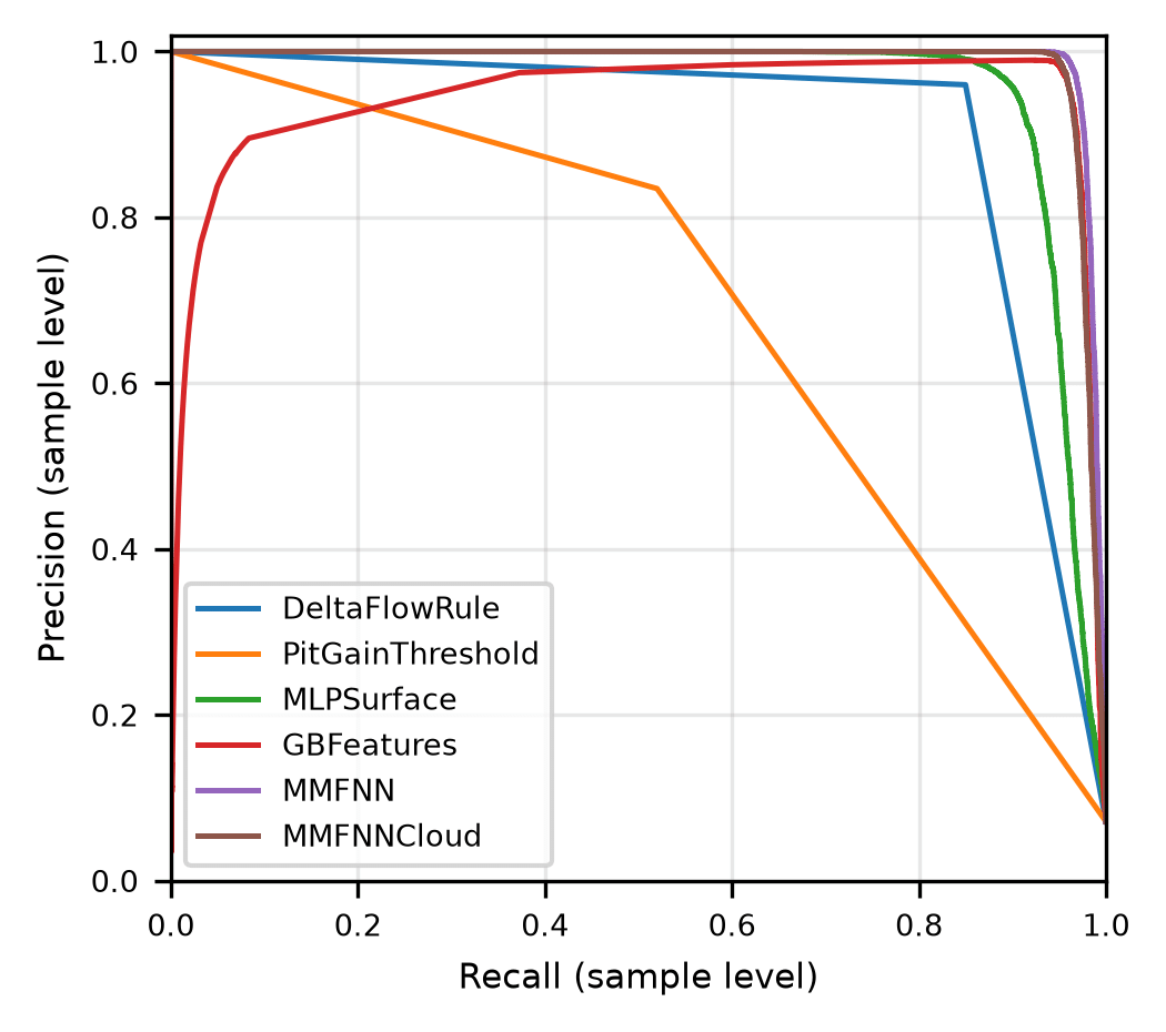
Figure 4: Precision–recall curves of the six detectors on the headline test set. Each curve pools all one-second samples. The two rule-based detectors give only 0 or 1, so their curves have a single corner. Colours are listed in the legend.
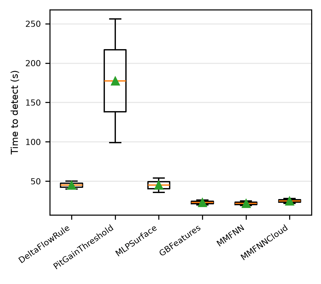
Figure 5: Time to detect for the kick scenarios each detector caught in the headline run. Boxes span the first to third quartile, the orange line is the median, the green triangle the mean, and whiskers reach 1.5 times the interquartile range.
6.2. Five Independent Replicates
A single test set of 37 kicks is a thin yardstick, since one missed scenario moves recall by almost three points. Table 5 therefore averages five independent replicates, 1,250 test scenarios and 185 kicks in all. The ordering of the headline run survives. The MMFNN has the lowest mean false-alarm rate, 0.8 ± 0.9 per 24 h, against 3.1 ± 1.6 for the gradient-boosted model and 20.0 ± 1.8 for the delta-flow rule. It also has the highest mean precision, 0.969 against 0.891.
The gap to the surface baselines is many standard deviations wide. The gap to the gradient-boosted model is smaller. The MMFNN had fewer false alarms in all five replicates and higher precision in all five replicates, and the mean paired difference is 2.3 ± 0.6 false alarms per 24 h (standard error). We read that as a likely advantage, not a settled one. On time to detect the two are tied, 23.5 s against 25.6 s, inside one standard deviation. Both are about twice as fast as the surface-only detectors, which sit near 45 s. Mean recall is 1.00 for the MMFNN and 0.96 for the delta-flow rule.
6.3. Channel Ablation
We removed channel groups and retrained the MMFNN, repeating the ablation in all five replicates (Table 6). Dropping the three downhole channels costs the most. Precision falls from 0.969 to 0.682, false alarms rise from 0.8 to 11.8 per 24 h, and median detection time roughly doubles, from 23.5 to 45.6 s. That is the case for downhole fusion in this simulator. DAS carries most of the benefit: without it precision drops to 0.815 and detection takes 34.4 s.
DTS and PWD behave differently, and we expected more from PWD. Removing either one leaves precision, false alarms and timing within about one standard deviation of the full model, and removing PWD even looks slightly better, though that difference amounts to a few false alarms over 1,065 non-kick scenarios. We do not read this as proof that PWD is useless in a real well. In the simulator a gas kick moves PWD by 15 to 55 psi (0.10 to 0.38 MPa) against a drift of up to 25 psi and noise of 15 psi. The channel is weak by construction, and the DTS sign is an assumption (Section 5.1). Two cautions follow. The gain here comes from the acoustic channel and the surface data, and DAS on a drillstring is far from routine, so the benefit rests on the least common sensor. And every statement about PWD and DTS is a statement about this simulator.
6.4. Probability Calibration
Monte-Carlo dropout is not implemented, so we cannot report calibration for the uncertainty head the design describes. What we can check is whether the MMFNN’s plain output probability can be trusted (Table 7 and Figure 6). The expected calibration error is very small, 0.0016 on average, and the Brier score of 0.0035 is the best of the learned detectors.
Table 5: Mean ± sample standard deviation over five independent replicates (1,250 test scenarios, 185 kicks, 178 h of non-kick drilling in total). MMFNN+MB is the mass-balance variant of Section 6.7. Other abbreviations as in Table 4.
| Method | Precision | Recall | AUPRC | FA/24 h | Median TTD (s) |
|---|---|---|---|---|---|
| DeltaFlowRule | 0.546 ± 0.030 | 0.96 ± 0.04 | 0.814 ± 0.016 | 20.0 ± 1.8 | 45.3 ± 5.6 |
| PitGainThreshold | 0.630 ± 0.034 | 0.95 ± 0.04 | 0.454 ± 0.020 | 13.9 ± 1.6 | 145.5 ± 20.6 |
| MLPSurface | 0.647 ± 0.072 | 0.95 ± 0.04 | 0.957 ± 0.004 | 13.3 ± 3.9 | 45.3 ± 7.4 |
| GBFeatures | 0.891 ± 0.051 | 0.99 ± 0.01 | 0.956 ± 0.009 | 3.1 ± 1.6 | 25.6 ± 3.3 |
| MMFNN | 0.969 ± 0.033 | 1.00 ± 0.00 | 0.985 ± 0.003 | 0.8 ± 0.9 | 23.5 ± 4.6 |
| MMFNNCloud | 0.969 ± 0.033 | 1.00 ± 0.00 | 0.979 ± 0.003 | 0.8 ± 0.9 | 26.5 ± 4.6 |
| MMFNN+MB | 0.946 ± 0.046 | 1.00 ± 0.00 | 0.984 ± 0.003 | 1.5 ± 1.3 | 24.7 ± 4.2 |
Table 6: Channel ablation of the MMFNN, mean ± standard deviation over five replicates. Abbreviations as in Table 4.
| Configuration | Precision | FA/24 h | Median TTD (s) |
|---|---|---|---|
| Full MMFNN | 0.969 ± 0.033 | 0.8 ± 0.9 | 23.5 ± 4.6 |
| No downhole (surface only) | 0.682 ± 0.109 | 11.8 ± 5.2 | 45.6 ± 10.0 |
| No DAS | 0.815 ± 0.093 | 5.8 ± 3.1 | 34.4 ± 10.2 |
| No DTS | 0.955 ± 0.040 | 1.2 ± 1.1 | 26.2 ± 4.6 |
| No PWD | 0.979 ± 0.022 | 0.5 ± 0.6 | 23.6 ± 4.0 |
| Only PWD + DAS | 0.937 ± 0.056 | 1.8 ± 1.6 | 28.9 ± 8.2 |
That headline number flatters the model. About 7 percent of samples are positive, and 99.5 percent of all samples fall in the two outermost bins, where predictions are easy. Only 802 samples, 0.5 percent, sit in the middle eight bins, and that is where the alarm decision is made. There the observed share of kick samples falls below the predicted probability, by 2 to 16 points between 0.4 and 0.9. The model is mildly over-confident exactly where it matters. A higher alarm threshold avoids that region (Section 6.6). The Monte-Carlo-dropout gate stays untested, so Table 1 still lists uncertainty gating as design only.
6.5. Sensitivity to Sensor Noise
The effect of PWD noise is best tested where PWD matters most, in a network that sees the surface channels plus PWD and no other downhole signal. We re-simulated both splits with the PWD noise standard deviation scaled from 0.05 to 8 times its nominal 15 psi (103 kPa), retrained, and scored five seeds each (Table 8).
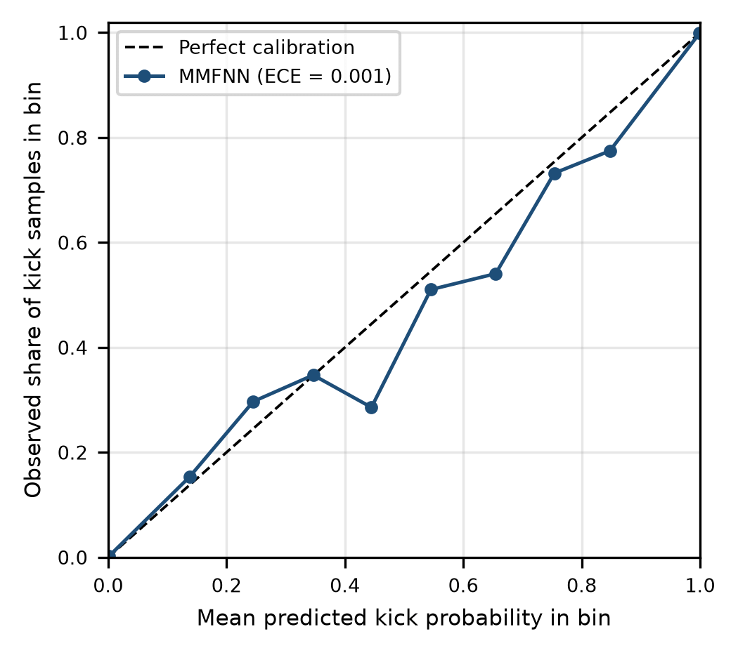
Figure 6: Reliability diagram of the MMFNN on the headline test set. Each point is one of ten equal-width probability bins; the dashed line is perfect calibration. The first and last bins hold more than 99 percent of the samples, and the points in between rest on few samples.
Table 7: Sample-level ranking and calibration, mean ± standard deviation over five replicates. ROC-AUC: area under the receiver operating characteristic; Brier: mean squared error of the probability; ECE: expected calibration error with ten bins.
| Method | ROC-AUC | Brier | ECE |
|---|---|---|---|
| MLPSurface | 0.9875 ± 0.0013 | 0.0088 ± 0.0009 | 0.0019 ± 0.0008 |
| GBFeatures | 0.9931 ± 0.0004 | 0.0044 ± 0.0001 | 0.0010 ± 0.0002 |
| MMFNN | 0.9957 ± 0.0011 | 0.0035 ± 0.0004 | 0.0016 ± 0.0007 |
| MMFNNCloud | 0.9937 ± 0.0012 | 0.0042 ± 0.0004 | 0.0023 ± 0.0007 |
| MMFNN+MB | 0.9956 ± 0.0013 | 0.0039 ± 0.0004 | 0.0021 ± 0.0005 |
Table 8: Surface channels plus PWD, with the PWD noise standard deviation scaled from its nominal 15 psi (103 kPa); mean ± standard deviation over five seeds. The last row repeats the surface-only network of Table 6. Column one gives the scale and, in brackets, the noise in kPa.
| PWD noise scale (kPa) | Precision | FA/24 h | Median TTD (s) |
|---|---|---|---|
| 0.05 (5) | 0.667 ± 0.027 | 12.0 ± 1.3 | 40.1 ± 15.0 |
| 0.1 (10) | 0.694 ± 0.067 | 10.8 ± 3.2 | 41.3 ± 14.4 |
| 0.25 (26) | 0.724 ± 0.085 | 9.5 ± 4.1 | 41.7 ± 11.2 |
| 0.5 (52) | 0.696 ± 0.069 | 10.7 ± 3.2 | 41.4 ± 11.1 |
| 1 (103) | 0.692 ± 0.077 | 11.1 ± 3.8 | 43.7 ± 8.4 |
| 2 (207) | 0.731 ± 0.075 | 9.2 ± 3.3 | 46.0 ± 8.8 |
| 4 (414) | 0.678 ± 0.057 | 11.5 ± 2.6 | 43.9 ± 6.8 |
| 8 (827) | 0.710 ± 0.064 | 9.9 ± 2.8 | 43.9 ± 6.3 |
| No PWD (surface only) | 0.682 ± 0.109 | 11.8 ± 5.2 | 45.6 ± 10.0 |
The result is flat. At nominal noise the surface-plus-PWD network reaches a precision of 0.692, no better than the surface-only network at 0.682, so PWD adds almost nothing here even before any extra noise is applied. Precision across the whole sweep stays between 0.667 and 0.731, inside the seed-to-seed scatter. In the full seven-channel network the same holds: with PWD noise at 120 psi (0.83 MPa) precision is 0.974, against 0.925 at nominal (one seed). Cutting the noise to 5 percent of nominal does not help either. What limits PWD here is probably not white noise at all. A kick moves the channel by 5 to 55 psi, the same order as its drift of up to 25 psi, and the sweep leaves that drift untouched. We have not isolated the drift effect, so this is a suspicion and not a finding. The network meanwhile learns to lean on the flow, pit and acoustic channels. The effect of PWD noise on precision in a real well remains open. Real PWD noise is neither white nor Gaussian, and a simulator in which PWD is strong would give a different answer.
Scaling the noise of every channel is a harsher test (Table 9). At twice the nominal noise the MMFNN loses some precision, 0.925 to 0.861, and its median detection time stretches from 22 to 30.5 s. It still beats the delta-flow rule on every metric. The gap to the gradient-boosted model does not survive, though. At that noise level GBFeatures has 2.0 false alarms per 24 h against 4.1 for the MMFNN in this single run. The MMFNN’s small advantage in Table 5 should not be assumed to hold when sensors are noisier than the training data.
6.6. Alarm Threshold and Network Latency
The 0.5 probability threshold and the three-sample debounce are defaults. We did not tune them on the test data. Table 10 shows what moving the threshold does on the headline run. Raising it from 0.5 to 0.9 removes all three false alarms and costs 2 s of detection time, while lowering it to 0.3 raises false alarms to 3.4 per 24 h. Because the middle probabilities are over-confident (Section 6.4), a higher operating point looks attractive, but it would have to be chosen on separate validation data and not on the test set shown here.
Network delay behaves as expected. Each second of round trip adds one second to the median time to detect, from 22 s with no delay to 32 s at 10 s, and precision does not move. AUPRC drops from 0.989 to 0.966, because a delayed probability lags the labels. Whether the delay matters operationally depends on what the driller can do with ten more seconds, which is outside what a simulator can say.
6.7. Mass-Balance Features as a Proxy for the Physics Terms
The loss in Section 4.4 cannot be trained with scikit-learn, so we tested a cheaper proxy. Two mass-balance features are appended to the seven channels before the rolling statistics are computed: the flow imbalance, outflow minus inflow, and the residual between that imbalance (in bbl/min) and the 30 s pit-gain rate. This is the MMFNN+MB row of Table 5.
The proxy brings no gain. Mean precision is 0.946 against 0.969 for the plain MMFNN, false alarms are 1.5 against 0.8 per 24 h, and median detection time is 24.7 s against 23.5 s. The plain network had fewer false alarms in three of five replicates and tied in one. The reason is probably structural. Flow imbalance and pit gain are generated from the same influx rate in (5) and (6), so the network already sees both and a residual between them adds little. Real wells differ, because measurement faults make a consistency check informative. This test says only that the simulator cannot show a benefit. The claim that physics constraints improve detection stays unproven here.
Table 9: Sensitivity to noise on every channel, one seed. Each cell gives precision / false alarms per 24 h, retrained at the stated noise scale; the last column is the MMFNN median time to detect.
| Noise scale | DeltaFlowRule | GBFeatures | MMFNN | MMFNN TTD (s) |
|---|---|---|---|---|
| 1 | 0.552 / 20.3 | 0.881 / 3.4 | 0.925 / 2.0 | 22.0 |
| 1.5 | 0.627 / 14.9 | 0.949 / 1.4 | 0.925 / 2.0 | 27.5 |
| 2 | 0.621 / 14.9 | 0.925 / 2.0 | 0.861 / 4.1 | 30.5 |
Table 10: Sweeps on the headline run (replicate 0). Upper block: alarm probability threshold with no network delay. Lower block: cloud round trip at the 0.5 threshold. Abbreviations as in Table 4.
| Setting | Precision | Recall | FA/24 h | Median TTD (s) |
|---|---|---|---|---|
| Threshold 0.3 | 0.881 | 1.00 | 3.4 | 22.0 |
| Threshold 0.5 | 0.925 | 1.00 | 2.0 | 22.0 |
| Threshold 0.7 | 0.974 | 1.00 | 0.7 | 23.0 |
| Threshold 0.9 | 1.000 | 1.00 | 0.0 | 24.0 |
| Round trip 0 s | 0.925 | 1.00 | 2.0 | 22.0 |
| Round trip 1 s | 0.925 | 1.00 | 2.0 | 23.0 |
| Round trip 3 s | 0.925 | 1.00 | 2.0 | 25.0 |
| Round trip 5 s | 0.925 | 1.00 | 2.0 | 27.0 |
| Round trip 10 s | 0.925 | 1.00 | 2.0 | 32.0 |
6.8. Compute Footprint Proxy
Table 11 reports the cost of the trained MMFNN on the development workstation. The network has 4,929 parameters, so one forward pass is about 9.9 kFLOPs, and the pickled model is 0.12 MB. A single-sample call takes 0.15 ms and a 60-sample batch 0.17 ms, figures probably dominated by scikit-learn call overhead rather than arithmetic. None of this is a Jetson Orin NX or Cortex-M7 measurement, and the rolling-statistics feature extraction is not included. The network itself is tiny. Whether the full pipeline, with INT8 quantisation, TensorRT and the OPC-UA stack, meets the latency target has to be measured on the gateway.
Table 11: CPU micro-benchmark of the MMFNN on a development workstation (a feasibility proxy, not a hardware-qualified result). FLOPs: floating-point operations, estimated as twice the parameter count.
| Metric | Value |
|---|---|
| Platform | Workstation CPU, scikit-learn |
| Latency, one sample (ms) | 0.152 |
| Latency, 60-sample batch (ms) | 0.175 |
| Model size, pickled (MB) | 0.122 |
| Parameters | 4,929 |
| FLOPs per inference | 9,858 |
7. Limitations and Deployment Considerations
Putting a model inside the drilling-safety loop raises questions that detection accuracy does not answer: hardware qualification, software assurance, drift, and who is responsible for the decision. The design keeps the alarm decision at the edge and leaves authority with the driller. It is decision support, not an autonomous controller.
The study has clear limits, and each one maps to work that has to be done before any field use:
- No real-well data. Everything ran on a simple simulator that leaves out wellbore storage, mud rheology, gas solubility, drillstring vibration and shut-in behaviour. The signature directions in Table 2 are assumptions, and the DTS direction is the weakest. The noise sweeps in Section 6.5 probe sensitivity but they are not a substitute for field logs or for cross-checks against OLGA or Drillbench.
- Only the MMFNN was trained. The transformer, the physics-informed loss, the Monte-Carlo-dropout gate and the explanation layer are designs. Section 6.7 tests a feature-level proxy for the mass-balance idea, which says little about the loss itself.
- No transfer learning. The pre-train and fine-tune protocol needs a real-well corpus that was not available, so the claim that ten real kicks would be enough is a target and not a result.
- No embedded measurement. The latency in Section 6.8 comes from a scikit-learn model on a workstation CPU. ONNX, INT8 and TensorRT on a Jetson Orin NX, and any Cortex-M7 downhole port, need their own benchmarks for latency, memory and power.
- Same-simulator training and testing. Even with five replicates, the training and test scenarios share the same generator, so the scores are an in-distribution upper bound.
- No human-factors work. The explanation layer has not been shown to drillers, and a structured operator study belongs in a field-pilot phase.
8. Conclusion and Future Work
We described an edge-AI architecture for kick detection in HPHT wells and tested one piece of it on an open simulator, a seven-channel feed-forward fusion network. Across five replicates it gave the lowest false-alarm rate (0.8 per 24 h) and the shortest median time to detect (23.5 s) of the six detectors. Against the surface rules the margin was large. Against a gradient-boosted model (3.1 false alarms per 24 h, 25.6 s) it was smaller, timing was tied, and the lead did not survive doubled sensor noise. Ablations pointed to the acoustic channel as the main source of the gain. The probabilities were reasonably calibrated but over-confident in the range that decides alarms. A 3 s cloud round trip cost 3 s of detection time.
These are simulator results, and the limits matter. The kick signatures are assumptions, the physics-informed loss was never trained, the transfer step was never run, and latency was timed on a workstation. The most useful next step is a comparison on real or commercial-simulator kicks. After that come implementing and ablating the physics-informed loss and the uncertainty gate, porting the model to a Jetson Orin NX with INT8 quantisation and timing the whole pipeline, and a pilot on a partner rig.
Appendix A: Physics Residuals for the Design-Level Loss
This appendix writes out the two residuals described in Section 4.4. They belong to the design and were not used in training. Let Qin and Qout be flow in and out (gpm), Vp the active pit volume (bbl), PPWD the downhole pressure (Pa), H the true vertical depth of the sensor (m) and g = 9.81 m/s². The network adds two auxiliary outputs next to the kick probability: an influx-rate estimate qθ,t (bbl/min) and an ECD deficit Δρθ,t (kg/m³).
Mud mass balance. Volume conservation says that the flow imbalance, converted to bbl/min with 42 gal per bbl, and the one-minute pit gain must both equal the influx the network claims,
Equivalent circulating density. The measured ECD follows from the PWD reading. The reference ECD adds a friction term from a fitted surrogate fφ of flow and standpipe pressure to the mud density ρm. A kick lowers the measured value below the reference by the deficit the network predicts,
Training objective. With a class-weighted binary cross-entropy LBCE, and scales σmb and σecd set from the noise level of each residual, the total loss is
where Lmb is the mean over t of [(rmb,t(1))² + (rmb,t(2))²] / σmb² and Lecd the mean of recd,t² / σecd². The weights λmb and λecd, the surrogate fφ and the scales are tuning choices that this study does not fix.
10. Data and Code Availability
The simulator, detectors, metrics, experiment runners and the result files behind every table and figure are provided as supplementary material. The headline run and the five replicates are reproducible from the stated seeds with run_experiments.py and run_extended.py.
11. Declaration of Generative AI Use
A generative AI assistant helped structure early drafts and suggest wording. AI-assisted coding tools were also used while writing parts of the simulator and experiment scripts. The author specified the architecture, the simulator physics, the experimental protocol and the metrics, ran and checked all code and results, and edited the text. The author takes full responsibility for the content of this paper.
12. Acknowledgment
The author thanks the associate editor and the three reviewers for comments that improved the manuscript.
- P. L. O’Bryan, A. T. Bourgoyne Jr., “Swelling of oil-based drilling fluids resulting from dissolved gas,” SPE Drilling Engineering, vol. 5, no. 2, pp. 149–155, 1990, doi:10.2118/16676-PA.
- National Academy of Engineering, National Research Council, Macondo Well Deepwater Horizon Blowout: Lessons for Improving Offshore Drilling Safety, Washington, DC, USA: National Academies Press, 2012, doi:10.17226/13273.
- American Petroleum Institute, API Recommended Practice 59: Recommended Practice for Well Control Operations, 2nd ed., Washington, DC, USA: API, 2006, reaffirmed May 19, 2023. [Online]. Available: https://www.apiwebstore.org/standards/59
- R. D. Grace, Blowout and Well Control Handbook, 2nd ed., Oxford, UK: Gulf Professional Publishing, 2017, doi:10.1016/C2016-0-03296-5.
- A. T. Bourgoyne Jr., K. K. Millheim, M. E. Chenevert, F. S. Young Jr., Applied Drilling Engineering, SPE Textbook Series, vol. 2, Richardson, TX, USA: Society of Petroleum Engineers, 1986, doi:10.2118/9781555630010.
- A. U. Osarogiagbon, F. Khan, R. Venkatesan, P. Gillard, “Review and analysis of supervised machine learning algorithms for hazardous events in drilling operations,” Process Safety and Environmental Protection, vol. 147, pp. 367–384, 2021, doi:10.1016/j.psep.2020.09.038.
- D. M. Nhat, R. Venkatesan, F. Khan, “Data-driven Bayesian network model for early kick detection in industrial drilling process,” Process Safety and Environmental Protection, vol. 138, pp. 130–138, 2020, doi:10.1016/j.psep.2020.03.017.
- S. Duan, X. Song, Y. Cui, Z. Xu, W. Liu, J. Fu, Z. Zhu, D. Li, “Intelligent kick warning based on drilling activity classification,” Geoenergy Science and Engineering, vol. 222, Art. no. 211408, 2023, doi:10.1016/j.geoen.2022.211408.
- C. Li, Z. Zhu, Y. Cui, H. Wang, Z. Xu, S. Duan, M. Zhou, “Intelligent kick warning model based on machine learning,” Processes, vol. 13, no. 7, Art. no. 2162, 2025, doi:10.3390/pr13072162.
- Q.-S. Yin, Z.-M. Yin, Z.-Q. Xu, M.-B. Li, L.-B. Zhang, J. Yang, D. Sui, Y.-Y. Guo, “Machine learning for gas kick detection in deepwater drilling: a review with multi-source data fusion,” Petroleum Science, vol. 23, no. 11, pp. 7187–7206, 2026, doi:10.1016/j.petsci.2026.06.012.
- A. H. Hartog, An Introduction to Distributed Optical Fibre Sensors, Boca Raton, FL, USA: CRC Press, 2017, doi:10.1201/9781315119014.
- R. Hutin, R. W. Tennent, S. V. Kashikar, “New mud pulse telemetry techniques for deepwater applications and improved real-time data capabilities,” in Proc. SPE/IADC Drilling Conference, Amsterdam, The Netherlands, 2001, doi:10.2118/67762-MS.
- M. Arifeen, A. Petrovski, M. J. Hasan, I. Kotenko, M. Sletov, P. Hassard, “DataDRILL: formation pressure prediction and kick detection for drilling rigs,” arXiv, arXiv:2409.19724, 2024, doi:10.48550/arXiv.2409.19724.
- B. Lim, S. Ö. Arık, N. Loeff, T. Pfister, “Temporal fusion transformers for interpretable multi-horizon time series forecasting,” International Journal of Forecasting, vol. 37, no. 4, pp. 1748–1764, 2021, doi:10.1016/j.ijforecast.2021.03.012.
- Y. Gal, Z. Ghahramani, “Dropout as a Bayesian approximation: representing model uncertainty in deep learning,” in Proc. 33rd International Conference on Machine Learning, Proceedings of Machine Learning Research, vol. 48, pp. 1050–1059, 2016. [Online]. Available: https://proceedings.mlr.press/v48/gal16.html
- Y. Ganin, V. Lempitsky, “Unsupervised domain adaptation by backpropagation,” in Proc. 32nd International Conference on Machine Learning, Proceedings of Machine Learning Research, vol. 37, pp. 1180–1189, 2015. [Online]. Available: https://proceedings.mlr.press/v37/ganin15.html
- S. M. Lundberg, S.-I. Lee, “A unified approach to interpreting model predictions,” in Advances in Neural Information Processing Systems 30, pp. 4765–4774, 2017. [Online]. Available: https://proceedings.neurips.cc/paper_files/paper/2017/hash/8a20a8621978632d76c43dfd28b67767-Abstract.html
- F. Pedregosa, G. Varoquaux, A. Gramfort, V. Michel, B. Thirion, O. Grisel, M. Blondel, P. Prettenhofer, R. Weiss, V. Dubourg, et al., “Scikit-learn: machine learning in Python,” Journal of Machine Learning Research, vol. 12, pp. 2825–2830, 2011. [Online]. Available: https://jmlr.org/papers/v12/pedregosa11a.html
- C. R. Harris, K. J. Millman, S. J. van der Walt, R. Gommers, P. Virtanen, D. Cournapeau, E. Wieser, J. Taylor, S. Berg, N. J. Smith, et al., “Array programming with NumPy,” Nature, vol. 585, no. 7825, pp. 357–362, 2020, doi:10.1038/s41586-020-2649-2.
No related articles were found.