
A Composite Technical Debt Index for Portfolio Risk Governance in Public-Sector Legacy Modernization

(This article belongs to the Section Software Engineering – Computer Science (SEC))
Export Citations
Cite
Managari, S. (2026). A Composite Technical Debt Index for Portfolio Risk Governance in Public-Sector Legacy Modernization. Journal of Engineering Research and Sciences, 5(11), 54–71. https://doi.org/10.55708/js0511004
Shivani Managari. "A Composite Technical Debt Index for Portfolio Risk Governance in Public-Sector Legacy Modernization." Journal of Engineering Research and Sciences 5, no. 11 (November 2026): 54–71. https://doi.org/10.55708/js0511004
S. Managari, "A Composite Technical Debt Index for Portfolio Risk Governance in Public-Sector Legacy Modernization," Journal of Engineering Research and Sciences, vol. 5, no. 11, pp. 54–71, Nov. 2026, doi: 10.55708/js0511004.
Technical debt in legacy modernization programs is currently evaluated at the level of individual code bases, with the results used to inform engineering executives about the technical priorities within their own systems, while the funding and sequencing of these activities are determined by program executives and boards on the basis of cross-system comparisons. This paper analyzes four technical-debt quantification methodologies SQALE, CAST-style structural measurement, static-analysis code-smell metrics, and defect-density modeling and explains the common limitation in all of these approaches: they define indicators fit for evaluation by a technical audience within one system but provide little guidance in comparing relative system scores and allocating resources among multiple systems under a common governance structure. The paper proposes the Composite Technical Debt Index (CTDI), a portfolio-level, governance-oriented index that combines four operational dimensions of technical debt interface fragility, documentation gaps, defect recurrence and batch/integration failure rates with change-activity attenuation, a separately reported service-criticality multiplier, and hard gates that escalate a system for review. CTDI is presented here as a testable research framework, not as a validated decision tool: the paper specifies the index precisely enough to be falsified and sets out the validation study that would test it. A hypothetical portfolio of four human-services systems illustrates how the index is computed and how its sensitivity is reported; in the illustration, a recently re-platformed payment system has a higher index value than the firm's COBOL mainframe, which would prioritize it for assessment. Whether it should receive more resources depends on remediation cost and expected risk reduction, which the illustration does not establish. As a research note, this paper does not offer empirical evidence for the superiority of CTDI over other approaches; rather, it specifies what falsification criteria would need to be established for a follow-up study to demonstrate such superiority over SQALE, CAST, or other technical-debt indexing methodologies.
1. Introduction
Large-scale legacy modernization programs in government and regulated industry routinely consume multi-year budgets and, with troubling regularity, overrun their schedules, exceed their cost envelopes, or fail at the seams between systems. Public audit bodies have repeatedly identified aging systems and their accumulated internal defects as a persistent source of operational and security exposure [1], [2]. Technical debt, the accumulated cost of expedient design and implementation choices [3], [4] is a widely accepted framing for the internal-quality component of that exposure.
The research literature on technical debt is substantial and increasingly mature. It offers taxonomies distinguishing code, architectural, documentation, test, and self-admitted debt [5], [6], [7] instruments for detecting and pricing debt items [8], [9], [10], [11] empirical evidence of debt’s cost in developer productivity [12] and systematic treatments of prioritization [13]. However, while this literature consistently addresses the engineering team, it rarely engages the governance layer. Detection and pricing instruments operate on one codebase and report in units remediation hours, violation counts, smell density meaningful to developers and architects. The decisions that determine whether debt is ever remediated in a modernization portfolio are made elsewhere: in funding cycles, sequencing decisions, and vendor negotiations conducted by executives who do not receive these units and could not compare them across a heterogeneous estate if they did.
Consequently, executives do not ignore technical debt; rather, they assess it through the only channel available to them: narrative vendor self-assessment, program-manager judgment, and the visible proxy of system age. Each of these is systematically biased. Vendors report on systems they are paid to maintain. Program managers are exposed to the debt that has recently caused an incident, not the debt that has not yet done so. System age is a poor proxy for delivery risk: the U.S. Government Accountability Office’s 2025 review of 69 federal legacy systems found the 11 most in need of modernization ranged from 23 to 60 years old, and age alone did not determine which systems were most critical [2]. Section 5 illustrates how CTDI would be computed for systems of different ages; it is not evidence that age is a poor proxy.
This paper addresses the translation problem. It makes five contributions.
- A portfolio-level, governance-oriented composite index (CTDI) that combines four operational technical-debt dimensions with change-activity attenuation, a service-criticality multiplier, and hard gates, in a single auditable rule (Section 4).
- A worked illustrative application showing how the index is computed, including a worked case for the change-activity and criticality terms and a full sensitivity analysis (Section 5).
- An example threshold table with a stated derivation and calibration procedure, so that others can compute the index (Section 4.2).
- A remediation-cost-per-unit-risk extension (ΔR/C) that connects the ranking to budget decisions (Section 6.6).
- A pre-registered validation protocol (Section 8) with a power discussion, model-comparison criteria, and falsification conditions, positioning CTDI as a testable research framework.
I state the paper’s principal limitation at the outset rather than deferring it. CTDI has not been applied to a real portfolio and its weights have not been calibrated against realized outcomes. The illustration in Section 5 is constructed using stipulated inputs; it does not show that the construct has predictive validity. Section 8 indicates what findings would provide evidence for the claim, including a naive baseline that CTDI must outperform if it is to lead to a transfer of funds. Those who look for a validated instrument will not find it here, but those who look for a specification that has been sharpened to a point at which it could be falsified will find it in abundance.
The four dimensions defined in Section 4 do not encompass all forms of technical debt: they do not cover, for example, test debt, requirements debt, architectural debt beyond interface fragility, data debt, or people/process debt (cf. [14], which identifies ten categories of technical debt at Google). A low CTDI score therefore does not mean a system has no technical debt it means it has low measured exposure on these four dimensions. CTDI must be used alongside code-level (SQALE/CAST) and test-coverage evidence, not as a replacement. The consequences of this limited coverage for decision-making are discussed in Section 6.5.
2. Related Work
The following review is in the form of a narrative and is therefore not systematic in nature. The review does not adhere to the systematic review protocol suggested by Kitchenham and Charters [15]. I make no claims of comprehensiveness in this review, because many of the works included in it provide the basis for developing the constructs used in this paper or describe the limitation addressed by this research. If the reader wants a systematic survey and analysis of the research area, the reader can refer to the mapping and review studies [6], [13], [16], [17].
2.1. Definition and Taxonomy
Cunningham’s original metaphor described the accumulating cost of shipping code that is not quite right [3]. Kruchten, Nord, and Ozkaya subsequently distinguished debt that is visible in artifacts from debt that is structural and invisible, and argued that the latter dominates long-run cost [4]. The Dagstuhl seminar on technical debt management consolidated terminology and produced the widely used distinction between debt items, their principal, and their interest [5]. Li, Avgeriou, and Liang’s systematic mapping catalogued the resulting taxonomy: requirements, design, architectural, code, test, build, documentation, infrastructure, and versioning debt [6].
Two of these categories are directly pertinent to modernization portfolios: architectural technical debt, which comprises decisions that were initially considered beneficial but have turned out to be liabilities [7], [18], [19], which tends to be the most challenging category to automatically detect, and which tends to be the most expensive; and documentation debt, which is often catalogued, but rarely quantified, since it is the factor most closely associated with legacy systems’ comprehension and therefore their replacement. Self-admitted technical debt, which takes the form of developer statements in source code comments, has been demonstrated to be detectable in an automated manner [20], and serves as a useful complement to the types of technical debt that are not amenable to static code analysis.
2.2. Quantification Approaches
Seaman and Guo used the finance domain to reason about debt measurement by analogy, suggesting tracking debt items with estimated principal and interest [8]. The SQALE method analysts utilized the analogies by defining the principal as the required remediation effort and subsequently calculating the ratio of the detected debt amount to the cost of complete redevelopment of the artifact [9]. Curtis, Sappidi, and Szynkarski estimated the principal on application level by assessing the number of structural violations impacting the codebase, which underpins the CAST family of products [10]. Nugroho, Visser, and Kuipers explicitly modeled interest in their framework by suggesting to consider the rate at which the codebase is modified as a factor affecting debt cost [11], which I employ explicitly in Section 4.4.
In [21], the authors evaluated four different approaches to debt identification on the same systems and found that they rarely identified the same code elements as debt items. This finding has bearing on my discussion because most composite approaches do not have a mechanism to reconcile the differences between the components. In fact, a composite approach would simply inherit all of the inconsistencies found in its components. In [17], the authors performed a systematic literature review to compare different financial analogies to technical debt and concluded that previous works inconsistently apply monetary terms to code debt.
2.3. Prioritization, Management, and Governance
Ernst and colleagues surveyed practitioners and found that architectural debt was the dominant concern while tooling attention was concentrated on code-level issues a mismatch between what is measured and what matters [22]. Rios and colleagues, in a global family of industrial surveys, identified deadline pressure and inadequate documentation among the most commonly reported causes and effects of debt [23]. Holvitie and colleagues documented practitioner perceptions of debt in agile settings across multiple countries [24].
Lenarduzzi and colleagues systematically reviewed technical debt prioritization and observed that most proposed approaches rank items within a single system and that empirical validation is scarce [13]. Avgeriou and colleagues, surveying the road ahead for debt management, named the integration of debt information into organizational decision-making as an open problem [25]. Ghanbari and colleagues examined practitioner perceptions of debt accountability, who is held responsible for debt they did not create which bears on the distributional questions I raise in Section 6.4 [26].
Behutiye and colleagues’ review of debt in agile development [16] and Besker, Martini, and Bosch’s quantification of productivity loss attributable to debt [12] together establish that debt has measurable organizational cost. Neither addresses the aggregation of that cost across an estate under multiple vendors.
2.4. Composite Indicator Construction
The technical debt literature has developed mostly in isolation from the considerable methodological literature on composite indicator construction, which this paper seeks to remedy. The OECD handbook on constructing composite indicators provides a canonical list of steps the theory of the case, choice of indicators, imputation, multivariate analysis, normalization, weighting and aggregation, analysis of uncertainty and sensitivity, decomposition, and links to other indicators together with a set of caveats concerning the ways in which the resulting indices can be misinterpreted [27]. Two of these warnings have particular relevance to the present discussion. First, normalizing to a distribution of countries, or other entities for example, percentile ranks renders the composite index non-comparable across time, since the reference distribution changes. Second, the choice of aggregation function determines whether the composite indicator is compensatory or not; that is, whether a given indicator can be “offset” by other indicators in the composite index, which is only appropriate when no indicator in the composite index is known to be fatal to the concept being measured.
Multi-criteria decision analysis approaches have been developed that address the two concerns raised by the OECD. Munda’s discussion of non-compensatory aggregation formalizes when weighted averaging procedures are inappropriate because of the presence of fatal indicators [28]. Saaty’s analytic hierarchy process, meanwhile, provides a canonical approach to determining preference weights for a given set of criteria based on paired comparisons, together with a formal consistency check [29]. Lastly, Strathern’s discussion of audit in higher education captures the sense in which an indicator becomes a target — particularly, when it is constructed using the inputs of those to be evaluated [30].
2.5. Recent Work, 2022–2025, and What CTDI Adds
Table 1 compares recent work (2022–2025) on technical-debt identification, measurement, and prioritization. No paper dated 2026 meeting the inclusion criteria for this table was found; the table therefore covers 2022–2025 and states that explicitly. Three patterns emerge. First, the field has moved toward holistic, context-aware, and empirically evaluated debt management: In [31], the authors report a shift toward a holistic approach, and [32] show debt assessed in context, with treatments fitted to sprint capacity. Second, tooling remains incomplete: In [33], the authors find that 59% of surveyed tools address management only, not identification or payment, and that empirical evaluation of self-admitted-debt tools shows low precision and recall. Third, code-level evidence continues to accumulate in [34] find code duplication and cognitive complexity the most frequently overlooked debt types in pull-request review, but none of the studies in Table 1 provides a portfolio-level governance index that combines operational dimensions with change-activity attenuation, service-criticality weighting, and hard gates in a single auditable rule. That is the gap CTDI addresses, as a testable framework.
What CTDI adds. The concrete additions over the approaches in Section 2.2 are: (1) SQALE (and SonarQube’s implementation of it) quantifies remediation cost in hours at code level and is size-normalized, but it has no portfolio-level governance layer, no service-criticality weighting, and no hard gate that escalates a system regardless of its score; (2) CAST-style structural measurement gives portfolio roll-up scores for structural quality, but it does not combine operational dimensions (interface fragility, batch/integration failure, documentation gap) with change activity and criticality in a single, auditable rule; (3) static-analysis code-smell approaches detect code-level smells, but they do not cover documentation, interface, or operational failure dimensions, and they do not produce a portfolio ranking; and (4) defect-density models measure observed defects per unit of code, which is a lagging outcome, whereas CTDI is a leading, multi-dimensional exposure index intended for prioritization before defects accumulate. CTDI’s contribution is therefore not a better code metric, but a governance index that is auditable (every input is a named proxy with a published threshold), portfolio-comparable (one tuple per system), and decision-linked (gates escalate; see Section 6.8). I state the limits of this comparison honestly: it is conceptual, because CTDI has not yet been validated against these approaches on the same portfolio — that head-to-head comparison is now a pre-specified part of the Section 8 protocol.
Table 1: Recent Work on Technical Debt, 2022–2025 Click to enlarge
| Year | Study | Approach / contribution | What CTDI adds |
|---|---|---|---|
| 2022 | [35] | Systematic review of 66 studies on requirements technical debt: identification and measurement are preliminary, with no consensus on measurement | CTDI does not measure requirements debt; it is scoped to four operational dimensions, and Section 6.5 states that limit explicitly |
| 2022 | [13] | Prioritization approaches proposed in research and industry; validated, reliable prioritization tools are lacking | CTDI is a prioritization index with a stated elicitation/calibration procedure (Section 4.10) and a pre-registered validation protocol (Section 8) |
| 2023 | [14] | Empirical, Google-based: ten categories of technical debt, measured by engineering surveys; tooling indicators alone do not capture context | CTDI’s four dimensions are a subset of these ten; Section 1 states that scope limit and uses the ten-category frame to define what CTDI does not cover |
| 2023 | [31] | Mapping update, 117 papers (2010–2022): more empirical evaluations; research focus shifting to a holistic approach | CTDI follows that holistic turn at portfolio level, combining dimensions, change activity, and criticality in one index |
| 2024 | [33] | Survey of 97 technical-debt tools; 59% address management only, not identification/payment; empirical evaluation of two self-admitted-debt tools shows low precision/recall | CTDI is not a tool; it is a governance index that can consume tool outputs (e.g. SQALE/CAST) as inputs, and its thresholds are published (Section 4.2) |
| 2025 | [32] | Observational case study: data debt and pipeline debt in data-intensive systems; debt assessed in context, treatments fitted to sprint capacity | Supports CTDI’s design choice to score dimensions in context and to report a tuple (score, gates, Unassessed status) rather than a single number |
| 2025 | [34] | Empirical study of 2,035 merged pull requests in 12 Apache projects (SonarQube) plus 250 review threads: code duplication and cognitive complexity most overlooked | Code-level evidence of the kind CTDI consumes as an input, not a substitute for portfolio governance |
| 2025 | [2] | Review of 69 federal legacy IT systems; 11 most in need of modernization (ages 23–60 years), scored on 16 attributes including age, vendor support, legacy languages, cybersecurity risk, and operating cost | The public-sector portfolio context for CTDI: GAO’s 16-attribute score is a precedent for a multi-attribute portfolio score, and CTDI’s four dimensions plus criticality and gates are presented as a complementary, auditable alternative, not a replacement |
Table 1: Recent Work on Technical Debt, 2022–2025
| Year | Study | Approach / contribution | What CTDI adds |
|---|---|---|---|
| 2022 | [35] | Systematic review of 66 studies on requirements technical debt: identification and measurement are preliminary, with no consensus on measurement | CTDI does not measure requirements debt; it is scoped to four operational dimensions, and Section 6.5 states that limit explicitly |
| 2022 | [13] | Prioritization approaches proposed in research and industry; validated, reliable prioritization tools are lacking | CTDI is a prioritization index with a stated elicitation/calibration procedure (Section 4.10) and a pre-registered validation protocol (Section 8) |
| 2023 | [14] | Empirical, Google-based: ten categories of technical debt, measured by engineering surveys; tooling indicators alone do not capture context | CTDI’s four dimensions are a subset of these ten; Section 1 states that scope limit and uses the ten-category frame to define what CTDI does not cover |
| 2023 | [31] | Mapping update, 117 papers (2010–2022): more empirical evaluations; research focus shifting to a holistic approach | CTDI follows that holistic turn at portfolio level, combining dimensions, change activity, and criticality in one index |
| 2024 | [33] | Survey of 97 technical-debt tools; 59% address management only, not identification/payment; empirical evaluation of two self-admitted-debt tools shows low precision/recall | CTDI is not a tool; it is a governance index that can consume tool outputs (e.g. SQALE/CAST) as inputs, and its thresholds are published (Section 4.2) |
| 2025 | [32] | Observational case study: data debt and pipeline debt in data-intensive systems; debt assessed in context, treatments fitted to sprint capacity | Supports CTDI’s design choice to score dimensions in context and to report a tuple (score, gates, Unassessed status) rather than a single number |
| 2025 | [34] | Empirical study of 2,035 merged pull requests in 12 Apache projects (SonarQube) plus 250 review threads: code duplication and cognitive complexity most overlooked | Code-level evidence of the kind CTDI consumes as an input, not a substitute for portfolio governance |
| 2025 | [2] | Review of 69 federal legacy IT systems; 11 most in need of modernization (ages 23–60 years), scored on 16 attributes including age, vendor support, legacy languages, cybersecurity risk, and operating cost | The public-sector portfolio context for CTDI: GAO’s 16-attribute score is a precedent for a multi-attribute portfolio score, and CTDI’s four dimensions plus criticality and gates are presented as a complementary, auditable alternative, not a replacement |
Portfolio-level decision making. Three further approaches belong in the comparison. Benchmark-based maintainability ratings (for example, the Software Improvement Group’s benchmark-based ratings) compare a system against a benchmark population but do not combine the result with criticality or gates. Application portfolio rationalization models notably Gartner’s TIME model (Tolerate, Invest, Migrate, Eliminate) sort applications by business value and technical fit but do not quantify technical-debt exposure within a system. Legacy modernization decision frameworks, including the GAO’s 2025 review [2], score systems on multiple attributes to decide disposition at portfolio level. CTDI is positioned as complementary to these: TIME- and GAO-style approaches decide disposition at portfolio level, while CTDI quantifies within-system exposure to inform that disposition.
3. Comparative Analysis and Design Requirements
Table 2 characterizes the four approaches along five governance-relevant attributes. The characterization is qualitative and derived from the published descriptions of each approach; it is not a scored benchmark, and no numeric ratings are asserted, because no common empirical basis for such ratings exists in the literature.
Characterization reflects each approach as described in the cited literature. Tool implementations vary and may extend beyond the published method.
Three observations follow. First, only CAST-style measurement was designed for portfolio roll-up, and its scoring model is proprietary, which makes it unsuitable as the basis of a decision an agency may be required to defend publicly. Second, the dimensions that practitioners identify as dominant architectural and documentation debt [22], [23] are the dimensions least covered by all four approaches. Third, none of the four specifies how its output should enter a funding decision; the translation is left entirely to the reader. I add a fourth observation, which weakens the “structural gap” argument as originally stated: Table 2 itself records that SQALE is size-normalized and that CAST supports portfolio roll-up, so the gap is not that these approaches cannot be compared across systems at all. The gap is that neither provides the governance outputs this paper argues are needed criticality weighting, change-activity attenuation, hard gates, and an Unassessed treatment — in one auditable rule (see Section 2.5).
From these observations, and from the methodological cautions in Section 2.4, I derive seven design requirements. I state explicitly that DR1–DR7 are derived from the same reasoning as the index, so meeting them is partly by construction: they are presented as design requirements (what the index was designed to satisfy), not as independent evidence that it succeeds. That evidence must come from the Section 8 validation.
- DR1 — Comparability. Scores must be comparable across systems differing in size, language, and architectural style.
- DR2 — Temporal stability. Normalization must be anchored to fixed, published thresholds, not to portfolio-relative statistics, so that a system’s score changes only when the system changes [27].
- DR3 — Limited compensability. One severe dimension must not be neutralized by three healthy ones [28].
- DR4 — Interest sensitivity. Identical debt in a frozen system and in a system under active change must not score identically [11].
- DR5 — Separation of magnitude from consequence. Debt magnitude and the consequence of failure must be reported independently — the consequence being determined by service criticality (Section 4.5), so that neither is masked by the other.
Table 2: Characterization of Established Quantification Approaches Along Governance-Relevant Attributes Click to enlarge
| Approach | Primary dimensions | Unit of analysis | Intended audience | Cross-system aggregation | Stated link to funding decisions |
|---|---|---|---|---|---|
| SQALE [9] | Remediation effort; maintainability violations | File to module; system debt ratio | Developer, architect | Ratio is size-normalized, so comparable in principle | None specified |
| CAST-style structural measurement [10] | Structural violations; estimated principal | Application, portfolio roll-up | Architect, IT executive | Supported; scoring model proprietary | Principal expressed in currency; sequencing not addressed |
| Static-analysis code smells | Smell density; duplication; complexity | Function, class, file | Developer | Not designed for it; density is size-sensitive | None |
| Defect-density models | Post-release defect rate | Module, release | QA, architect | Comparable only at equal exposure | Indirect, via quality gates |
Table 2: Characterization of Established Quantification Approaches Along Governance-Relevant Attributes
| Approach | Primary dimensions | Unit of analysis | Intended audience | Cross-system aggregation | Stated link to funding decisions |
|---|---|---|---|---|---|
| SQALE [9] | Remediation effort; maintainability violations | File to module; system debt ratio | Developer, architect | Ratio is size-normalized, so comparable in principle | None specified |
| CAST-style structural measurement [10] | Structural violations; estimated principal | Application, portfolio roll-up | Architect, IT executive | Supported; scoring model proprietary | Principal expressed in currency; sequencing not addressed |
| Static-analysis code smells | Smell density; duplication; complexity | Function, class, file | Developer | Not designed for it; density is size-sensitive | None |
| Defect-density models | Post-release defect rate | Module, release | QA, architect | Comparable only at equal exposure | Indirect, via quality gates |
- DR6 — Explicit treatment of the unquantified. The systems that have not been quantified must be assigned a unique treatment and must never be assigned a default or portfolio-average value, since the application of a mean value to an unquantified legacy system could substantially underestimate the risk concentration in that system [27].
- DR7 — Resistance to strategic reporting. Because much input data originates with the vendors being evaluated, the construct must anticipate optimization of the measure [30].
4. The Composite Technical Debt Index
Figure 1 shows the construct’s computation path. Two features of the diagram carry the design argument. The scored path runs down the center: raw proxies are normalized, aggregated, attenuated by change activity, and scaled by criticality. Gate evaluation and coverage checking run beside it and never enter the arithmetic, because both express conditions that averaging would misrepresent. The output is accordingly a tuple rather than a number.
4.1. Dimensions
CTDI uses four debt dimensions. Each was selected because it appears in the reviewed literature, is observable without instrumenting source code the assessing organization may not control, and is meaningful to a non-technical decision-maker. Table 3 gives definitions and candidate proxies. I denote the dimensions d = 1, …, 4 in the order of Table 3: interface fragility (IF), documentation gap (DG), defect recurrence (DR), and batch/integration failure rate (BIF).
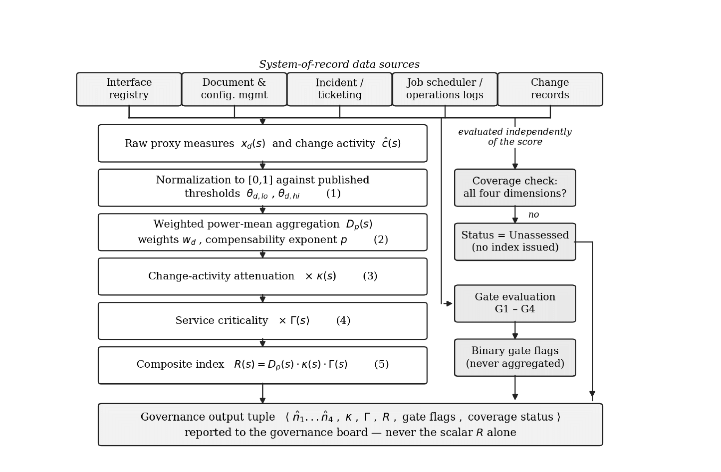
Table 3: CTDI Debt Dimensions, Definitions, and Candidate Proxies Click to enlarge
| Dimension | Definition | Candidate proxy measures | Typical source |
|---|---|---|---|
| Interface fragility (IF) | Susceptibility of the system’s external boundaries to breakage under change | Count of undocumented or unversioned interfaces; share of interfaces without contract tests; breaking-change rate per release | Interface inventory; release records |
| Documentation gap (DG) | Extent to which system behavior cannot be reconstructed from written artifacts | Share of modules without current design documentation; age of newest architecture document; share of business rules existing only in code | Configuration management; document review |
| Defect recurrence (DR) | Degree to which defects reappear rather than being resolved | Share of incidents that are reopens or recurrences of a prior root cause within a defined window | Incident and ticketing system |
| Batch/integration failure rate (BIF) | Frequency with which scheduled or inter-system processing fails to complete correctly | Failed or late batch cycles as a share of scheduled cycles; reconciliation exception rate | Operations logs; job scheduler |
Table 3: CTDI Debt Dimensions, Definitions, and Candidate Proxies
| Dimension | Definition | Candidate proxy measures | Typical source |
|---|---|---|---|
| Interface fragility (IF) | Susceptibility of the system’s external boundaries to breakage under change | Count of undocumented or unversioned interfaces; share of interfaces without contract tests; breaking-change rate per release | Interface inventory; release records |
| Documentation gap (DG) | Extent to which system behavior cannot be reconstructed from written artifacts | Share of modules without current design documentation; age of newest architecture document; share of business rules existing only in code | Configuration management; document review |
| Defect recurrence (DR) | Degree to which defects reappear rather than being resolved | Share of incidents that are reopens or recurrences of a prior root cause within a defined window | Incident and ticketing system |
| Batch/integration failure rate (BIF) | Frequency with which scheduled or inter-system processing fails to complete correctly | Failed or late batch cycles as a share of scheduled cycles; reconciliation exception rate | Operations logs; job scheduler |
These four are neither exhaustive nor independent. Interface fragility and batch failure rate will correlate in most estates, and the OECD guidance is explicit that correlated components should be examined by multivariate analysis before weights are assigned [27]. Section 4.11 treats this as a construct-validity question, and Section 7 as a limitation.
4.2. Normalization
For system s and dimension d, let x_d(s) be the raw proxy measure. Two fixed thresholds are published in advance: θ_{d,lo}, the value at or below which the dimension is considered acceptable, and θ_{d,hi}, the value at or above which it is considered severe. The normalized value is the clipped linear interpolation between them:
so that n̂_d(s) ∈ [0, 1] with higher values indicating worse condition. Anchoring to published thresholds rather than to the portfolio’s own distribution satisfies DR2: a system’s normalized score does not change because another system in the portfolio improved. Thresholds should be set from documented operational tolerances where these exist and revisited on a fixed schedule, with the revision date recorded, since silently re-anchoring thresholds is equivalent to rewriting history.
Worked example. Take the documentation gap of the illustrative payment system S3 in Section 5. Its raw proxy is 47.5% of modules without current design documentation. With the example thresholds in Table 4 (θ_lo = 10%, θ_hi = 60%), the normalized value is (47.5 − 10) / (60 − 10) = 0.75, which is the DG value used for S3 in Table 6. A reader with the raw proxy and Table 4 can recompute every normalized input in the same way.
Example thresholds. Table 4 gives example threshold values for every proxy, for the change-activity measure, and for the criticality rubric. The table is labeled example/illustrative, not empirically derived: the values are starting points for calibration, not findings. Without published thresholds, nobody else can compute the index; with them, any reader can. Section 4.14 states how the thresholds would be set and re-calibrated.
4.3. Aggregation with Adjustable Compensability
Debt dimensions are aggregated by a weighted generalized power mean
The exponent p governs compensability. At p = 1 the function is the weighted arithmetic mean and dimensions substitute freely for one another. As p increases the function is progressively dominated by its largest argument, approaching the maximum as p → ∞. This single parameter therefore expresses a governance judgment that is otherwise left implicit: how far a serious failing in one dimension may be offset by strength elsewhere. I recommend p = 2 as a default and require that results be reported with the sensitivity analysis of Section 4.8, because as Section 5 shows, p can change a system’s governance disposition.
Selecting p > 1 addresses DR3 but does not eliminate compensability. Dimensions capable of independently ending a program are not handled by the aggregation function at all; they are handled by the gates of Section 4.6.
Table 4: Example Threshold Values (Illustrative Starting Points for Calibration, Not Empirically Derived Values) Click to enlarge
| Proxy | θ_lo (score 0) | θ_hi (score 1) | How the example value was chosen |
|---|---|---|---|
| Interface fragility (IF): proportion of undocumented or unversioned interfaces | 5% | 40% | Illustrative thresholds selected for the worked example. These values are not established SIG/SonarQube benchmarks and require calibration using interface audit data and expert assessment. |
| Documentation gap (DG): proportion of modules without current design documentation | 10% | 60% | Illustrative thresholds based on expert judgment. Proposed calibration through the Delphi procedure described in Section 4.10. |
| Defect recurrence (DR): reopened or recurring incidents per 100 incidents | 5 per 100 | 30 per 100 | Illustrative thresholds based on assumed incident recurrence levels. Calibration requires historical incident records and consistent recurrence definitions. |
| Batch/integration failure rate (BIF): failed or late cycles per 100 scheduled cycles | 1 per 100 | 15 per 100 | Illustrative thresholds representing low and high operational failure rates. Calibration requires recorded batch and integration outcomes. |
| Change activity ĉ: normalized change rate | 0.1 | 0.9 | Illustrative low and high normalized change-activity values. Normalization should use fixed, documented reference thresholds to preserve comparability across reporting periods. The attenuation floor is κ_min = 0.4 floor |
| Service criticality: affected population | 100 (lowest band) | 10,000 (highest band) | Illustrative population bands of 100, 1,000, and 10,000 people. The portfolio owner and service owners must define the band boundaries and explain how affected population contributes to the service-criticality assessment. |
Table 4: Example Threshold Values (Illustrative Starting Points for Calibration, Not Empirically Derived Values)
| Proxy | θ_lo (score 0) | θ_hi (score 1) | How the example value was chosen |
|---|---|---|---|
| Interface fragility (IF): proportion of undocumented or unversioned interfaces | 5% | 40% | Illustrative thresholds selected for the worked example. These values are not established SIG/SonarQube benchmarks and require calibration using interface audit data and expert assessment. |
| Documentation gap (DG): proportion of modules without current design documentation | 10% | 60% | Illustrative thresholds based on expert judgment. Proposed calibration through the Delphi procedure described in Section 4.10. |
| Defect recurrence (DR): reopened or recurring incidents per 100 incidents | 5 per 100 | 30 per 100 | Illustrative thresholds based on assumed incident recurrence levels. Calibration requires historical incident records and consistent recurrence definitions. |
| Batch/integration failure rate (BIF): failed or late cycles per 100 scheduled cycles | 1 per 100 | 15 per 100 | Illustrative thresholds representing low and high operational failure rates. Calibration requires recorded batch and integration outcomes. |
| Change activity ĉ: normalized change rate | 0.1 | 0.9 | Illustrative low and high normalized change-activity values. Normalization should use fixed, documented reference thresholds to preserve comparability across reporting periods. The attenuation floor is κ_min = 0.4 floor |
| Service criticality: affected population | 100 (lowest band) | 10,000 (highest band) | Illustrative population bands of 100, 1,000, and 10,000 people. The portfolio owner and service owners must define the band boundaries and explain how affected population contributes to the service-criticality assessment. |
Table 5: Hard Gate Conditions Reported Independently of the Index Click to enlarge
| Gate | Condition | Rationale |
|---|---|---|
| G1 Supportability cliff | Runtime, compiler, database, or hardware platform past vendor end-of-support, or with end-of-support inside the planning horizon | Risk is a dated discontinuity, not a gradient; remediation timing is externally imposed |
| G2 Irreproducible build | System cannot be rebuilt from controlled sources by the current custodian | Modernization cannot be planned for an artifact that cannot be reconstructed |
| G3 Unmitigated vendor concentration | Single supplier holds exclusive operational knowledge with no escrow or transition plan | Exposure is contractual, not technical, and is invisible to code metrics |
| G4 Exposed unpatched vulnerability | Known exploitable defect reachable from an untrusted network and not remediable within the maintenance regime | Security exposure is not tradable against maintainability |
Table 5: Hard Gate Conditions Reported Independently of the Index
| Gate | Condition | Rationale |
|---|---|---|
| G1 Supportability cliff | Runtime, compiler, database, or hardware platform past vendor end-of-support, or with end-of-support inside the planning horizon | Risk is a dated discontinuity, not a gradient; remediation timing is externally imposed |
| G2 Irreproducible build | System cannot be rebuilt from controlled sources by the current custodian | Modernization cannot be planned for an artifact that cannot be reconstructed |
| G3 Unmitigated vendor concentration | Single supplier holds exclusive operational knowledge with no escrow or transition plan | Exposure is contractual, not technical, and is invisible to code metrics |
| G4 Exposed unpatched vulnerability | Known exploitable defect reachable from an untrusted network and not remediable within the maintenance regime | Security exposure is not tradable against maintainability |
4.4. Change-Activity Attenuation
Debt has a cost when the system is changed [11]. A frozen, poorly performing system is a supportability and knowledge risk, but not the same kind of delivery risk as one that is poorly performing and is changed weekly. Let ĉ(s) ∈ [0, 1] be a normalized measure of recent change activity. For a trailing window of change requests, releases, or commits per unit time, this is the count normalized against a threshold, as in equation (1). Define
with κ_min = (0, 1] being a minimum fraction representing how much of the debt of the static system is relevant. I set κ_min = 0.4. The threshold should not be set to zero, as that would imply that frozen systems do not pose any risk to the ongoing operations, which is incorrect as they fail supportability and staff retention rather than change-related problems. This satisfies DR4. The risks of this form including that it discounts frozen systems and penalizes systems under active remediation are discussed in Section 4.13.
4.5. Service Criticality
Debt magnitude and the consequences of its failure are separate measurements represented in different scales according to DR5. The criticality is determined by a published criterion that includes four features presented as true or false. Four features are as follows: the number of affected people is above a given minimum, interruption causes denial or delay of a benefit mandated by a regulation instead of an administrative hassle, there is no manual process that can handle the normal volume, and the system has a vulnerability to statutory or judicial deadlines. Using the number of features, f, for the system, where f ∈ {0, 1, 2, 3, 4}:
Why is criticality a multiplier rather than a fifth weighted dimension? Because a low-criticality system with extreme debt is a different problem than a high-criticality system with low debt; the two should not be aggregated as if they have the same impact on the business. The rubric deliberately focuses on harm from interruption rather than transactions or budget because criticality based on unit volume would punish systems that serve few users (Section 6.4).
The composite index is then
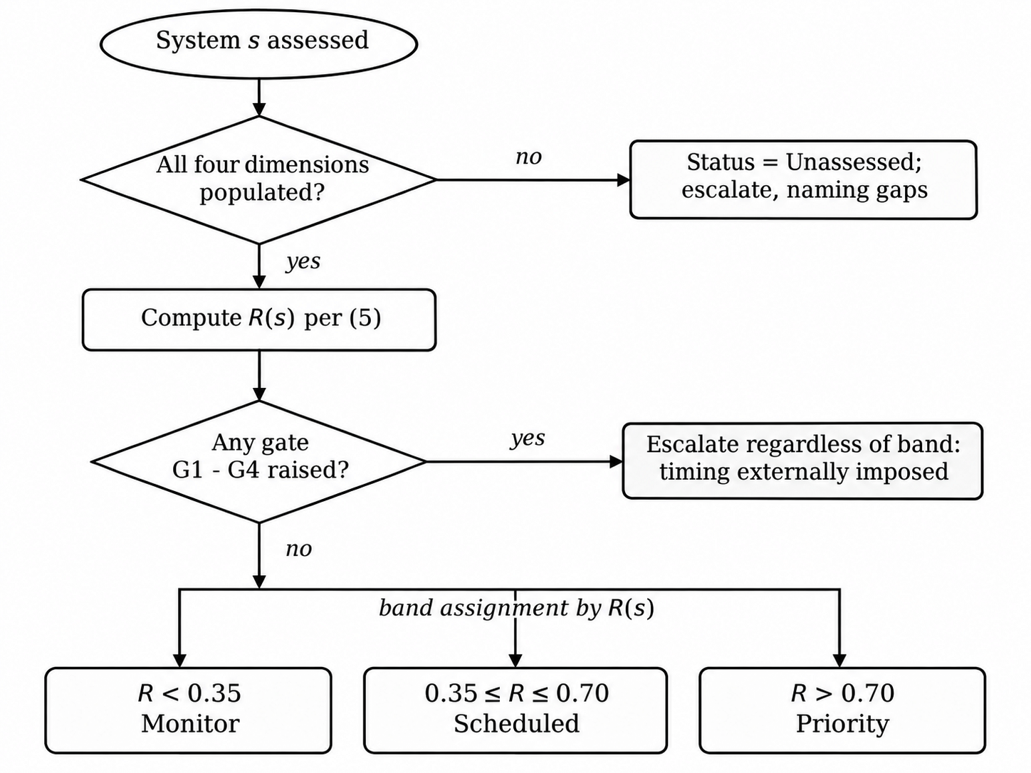
with indicative bands R < 0.35 (monitor), 0.35 ≤ R ≤ 0.70 (scheduled remediation), and R > 0.70 (priority remediation). These bands are for illustration only and should be set according to the organization’s own results before taking any action. Section 4.16 explains how to interpret R, including values above 1.0.
4.6. Hard Gates
Certain types of risk to a system are of such a nature that they are either entirely avoided or fundamentally altered and are therefore not incremental in the way that the index suggests. Table 5 lists gate conditions that are reported as binary flags along with R and are therefore not incorporated into the calculation in equation (5). Any raised gate is an issue of concern to the authorities, regardless of the value of the index.
4.7. Coverage and Unassessed Status
Per DR6, a system is scored only if at least three of the four dimensions can be populated (minimum coverage 3/4). If one dimension is missing, the score is reported as a range best case, with the missing dimension set to 0, and worst case, with it set to 1 together with the width of that range, so that a reader can see how much the missing data matters (see Section 5.4 for the worked ranges). If two or more dimensions are missing, the system receives status Unassessed and no index value. Unassessed status is itself reported to the governance board as an open item with the specific missing dimensions named, and an Unassessed system is treated as more critical for governance purposes it is escalated for assessment, not silently ranked low (see also Section 6.4). This rule exists because the alternatives are worse: imputing the portfolio mean makes the least-instrumented systems appear average, and imputing zero makes them appear healthy. In most public-sector estates the least-instrumented systems are the oldest and the most consequential, so both defaults would produce exactly the misallocation the construct is intended to prevent. Because the documentation gap relies on human judgment, the most important legacy systems — those with the least documentation — are the most likely to be Unassessed, so an Unassessed list must be reviewed by the portfolio board as a priority list in its own right, not filed away.
Figure 2 gives the resulting disposition logic. Coverage failure and a raised gate both short-circuit band assignment, which is the operational expression of the argument that a scalar index must not be the sole determinant of governance attention. Note the order in Figure 2: R is computed before the gates are applied; a raised gate then escalates the system regardless of its band.
4.8. Sensitivity Analysis
Any reported CTDI result must be accompanied by a sensitivity analysis over (i) the weight vector, sampled over the simplex, (ii) the exponent p, (iii) the attenuation floor κ_min, (iv) the criticality step, and (v) the band edges. A ranking that does not survive such an analysis is an artifact of the analyst’s choice of parameters and should not be reported to the decision-maker. This section states the requirement; Section 5.3 reports the analysis, recomputed from the manuscript’s own formulas (2)–(5) and the stipulated inputs of Table 6, for the illustrative example. The headline result is stated here because it governs how the example may be reported: the S1/S4 ranking does not survive variation in p, and it is therefore withdrawn as a finding.
4.8.1. Method
All sensitivity computations use equal weights (w_d = 0.25) and the baseline parameters p = 2, κ_min = 0.4, criticality step 0.2, and band edges 0.35/0.70 unless the parameter under study is varied. Weights are sampled over the simplex by Dirichlet sampling (1,000 draws, seed 7, for reproducibility), together with the four one-dimension-dominant corners (one weight 0.7, the others 0.1). p is varied over {1, 1.5, 2, 3}; κ_min over {0.0, 0.2, 0.4, 0.6}; the criticality step over {0.1, 0.2, 0.3}; and the band edges are shifted by ±10% (0.315/0.63 and 0.385/0.77). No new data are introduced: the analysis varies only the parameters of the framework applied to the same stipulated inputs.
4.9. Parameter Defaults and Their Status
The parameters of the framework are stipulated defaults, not empirically established values, and the manuscript now says so for each of them. p = 2 is the Euclidean (L2) default, chosen because it penalizes a system that is very bad on one dimension more than a simple average would, while remaining the standard, least arbitrary choice among L_p norms. κ_min = 0.4 is a floor chosen so that a frozen system is discounted but never erased (see Section 4.13 for the discussion of its risks). The criticality multiplier uses a 0.2 step per criticality band, chosen as a transparent, linear default that can be read off the rubric. The normalization thresholds θ_lo/θ_hi are the example values in Table 4, to be calibrated as described in Section 4.14. The band edges 0.35 and 0.70 are illustrative. Section 4.8 and Section 5.3 show how the ranking moves when each of these values changes, so a reader can see exactly which conclusions depend on which stipulation. No parameter is presented as empirically established.
4.10. Weight Elicitation and Calibration
Equal weights (w = 0.25 per dimension) are kept as the initial recommendation and are described throughout as the transparent starting point, not a finding. The structured procedure for deciding weights is as follows.
A Delphi round with portfolio architects, service owners, and maintainers, scoring the relative importance of the four dimensions.
Conversion of the Delphi judgments to weights by the Analytic Hierarchy Process (AHP), with a consistency-ratio check (CR < 0.10) and a documented fallback to equal weights if consistency is not achieved [29].
Held-out calibration in the Section 8 validation study, in which weights are fitted on one half of the portfolio and tested on the other, so that any fitted weights must generalize out of sample. The construct provides no principled basis for the weights absent calibration against outcomes; equal weighting is the defensible default when no evidence distinguishes the dimensions, and the OECD guidance notes that it is often mistaken for the absence of a weighting decision when it is in fact a substantive one [27].
4.11. Construct Validity: Correlation and Double-Counting
Interface fragility (dimension 1) and batch/integration failure rate (dimension 4) are plausibly correlated, because fragile interfaces fail in batch and integration, so a system could be counted twice for what is partly one underlying weakness. The manuscript itself identifies this as a construct-validity concern and addresses it in three ways.
The four dimensions are defined in Section 4.1 with non-overlapping measurement rules: interface fragility is measured from interface inventory, contract/version, and dependency evidence, while batch/integration failure is measured from observed failure rates in batch and integration runs, so the same event is not counted in both.
The validation protocol (Section 8) now requires reporting the inter-dimension correlation matrix on the real portfolio and, if any pair exceeds a pre-specified threshold (r > 0.70), re-estimating the index with the correlated dimensions merged or down-weighted and reporting both versions.
The sensitivity analysis (Section 4.8) samples weights across the simplex, which shows how much the ranking depends on the weight given to either of the two correlated dimensions (Section 5.3). Until that correlation is measured, rankings driven mainly by dimensions 1 and 4 should be treated as provisional (see Section 6).
4.12. What CTDI Indexes — and What It Does Not
CTDI is, as constructed, a risk-priority-weighted exposure index: it combines operational risk indicators (the four dimensions, which proxy the likelihood of delivery or operational failure) with change activity and service criticality (which proxy consequence). It is not a measure of financial principal (the cost to remediate all debt) or interest (the ongoing cost of carrying it), even though Section 2 discusses principal and interest as the conceptual background. I have kept the name “Composite Technical Debt Index” because the four dimensions are technical-debt indicators and the index is used for technical-debt governance, but the manuscript now defines the name in that qualified sense in the abstract, in Section 1, and here, and it no longer implies that R is a principal or interest figure. Allocating resources needs remediation cost (or risk reduction per unit cost), which a ranking by R alone cannot provide; that extension is given in Section 6.6.
4.13. Attenuation: Risks and Limits
I do not have evidence for κ_min = 0.4 or for the linear form in equation (3), and I say so: both are stipulated defaults, chosen for transparency (a linear form that any reader can recompute), not on empirical evidence. Three risks are stated here. (i) A frozen system is discounted to 40% even though its knowledge and documentation risk matters most when it is about to be replaced; κ must therefore not be applied to the documentation-gap dimension in a way that hides it, and a frozen system with a high documentation gap still raises the relevant gate. (ii) The form rewards freezing change and penalizes active remediation: S3 scores high partly because it is being re-platformed, and Section 5 now says so, rather than presenting S3’s score as a pure debt signal. (iii) ĉ is easy to game (a team can suppress recorded change activity); ĉ must therefore be computed from version-control and deployment logs, not from self-report, and the source of ĉ must be recorded alongside the score. The sensitivity analysis (Section 4.8) varies κ_min across {0.0, 0.2, 0.4, 0.6} so that a reader can see how much any conclusion depends on the 0.4 floor. A non-linear attenuation form is listed as future work in Section 8.
4.14. Setting Thresholds
Thresholds are set in three steps.
Anchor to a published band where one exists (SQALE/SIG maintainability bands, SonarQube quality-gate defaults).
Adjust by Delphi with the portfolio’s architects and service owners.
Re-calibrate on the first real portfolio in the Section 8 validation study, with the calibrated values published alongside the results. Until step (3) is done, Table 4 is an example, and the manuscript says so. Thresholds are revisited on a fixed schedule, with the revision date recorded (Section 4.2).
4.15. Hard Gates: Thresholds and Evidence
Each gate in Table 5 is stated with its threshold, the reason for that threshold, and its status. The thresholds are stipulated defaults, chosen so that a gate fires only on a severe single-dimension failure. For example, G1 (supportability cliff) fires when a platform is past vendor end-of-support or has end-of-support inside the planning horizon — in the illustrative example, the COBOL mainframe S1 raises G1 for that reason, not because of its documentation-gap score. I do not have supporting evidence for the gate thresholds, and I say so; the validation protocol (Section 8) requires reporting the gate firing rate and the outcomes of gated versus non-gated systems, so that the thresholds can be calibrated. Gates escalate a system for review; a gated system is not “not considered for continued operation” (see Section 5.5).
4.16. Interpreting R, Including Values Above 1.0
The dimension aggregate D is normalized to [0, 1]; κ is in [κ_min, 1]; Γ is ≥ 1, so R = D × κ × Γ can exceed 1.0. The value above 1.0 is the criticality multiplier, not a probability and not a percentage: it means the system’s exposure is amplified by its criticality. The indicative bands of Section 4.5 apply: R < 0.35, monitor; 0.35 ≤ R ≤ 0.70, scheduled remediation; R > 0.70, priority remediation; and R ≥ 1.0 is high exposure on a critical service, escalated regardless of the exact value. These bands are illustrative and should be set by the organization before use. The tuple (R, gates, Unassessed status) is always reported together, so a system with R = 0.30 that has raised a gate is escalated, while a system with R = 0.90 and no gate is prioritized but not gated. R is not a measure of principal or interest (Section 4.12).
5. Illustrative Application
It is a hypothetical example; this portfolio, these inputs, and these scores have been specified by me to demonstrate the mechanism of the construct. There is no implication that any particular agency, system, or procurement decision is described here, nor is anything in this section intended to be evidence of CTDI’s ability to predict delivery outcomes. The example demonstrates how the mechanism operates; it cannot establish validity, predictive power, or superiority.
Imagine a human-services portfolio of four information systems undergoing phased modernization. S1 is an eligibility-determination COBOL mainframe application that has been functionally frozen for replacement. S2 is a midlife client-server case-management application with moderate requirements for change. S3 is a payment-disbursement system that has been re-platformed to distributed services in the past eighteen months and is now subject to intense change. S4 is a correspondence/print-fulfillment system that is small and stable, but its nightly production batch to an outside print vendor is failing frequently. Table 6 specifies the normalized inputs for this hypothetical scenario.
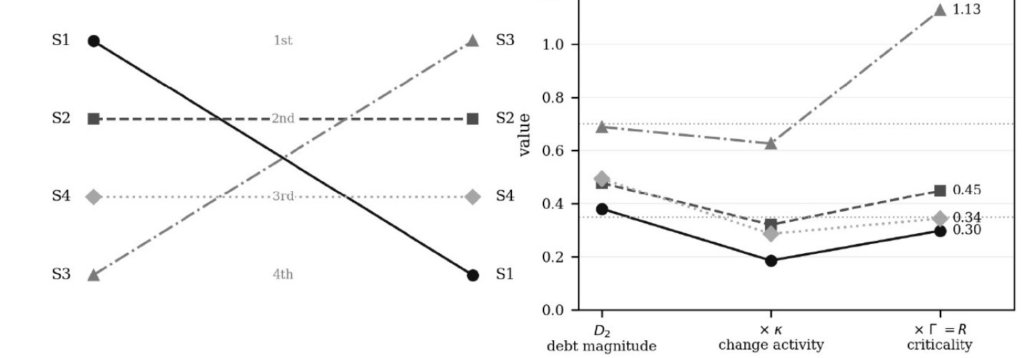
Applying equations (2) through (5) with equal weights and p = 2 yields the results in Table 7. The given order is R: S3 (1.127), S2 (0.449), S4 (0.344), S1 (0.298). This is the opposite of the order based on the system age and architectural vintage, which would intuitively be expected to be the COBOL mainframe first, then the more recently re-platformed payment system last. It is precisely the point of the example that it is the opposite as an illustration of the mechanism, not as evidence about real systems. The mainframe has a documentation gap DG = 0.55 and has raised the G1 supportability gate and is therefore escalated despite its other scores; it is not a system with “little debt of any kind.” The payment system, by contrast, has a set of fragile interfaces, inadequate documentation for a system that is in the midst of a significant re-platforming, frequent reconciliation errors, extensive change exposure, and highest at-risk consequence in case of interruption and hence ranks first in Table 7. A governance board considering only the architectural vintage would not only fund the mainframe but most likely be surprised by the risk discovery on the payment system. Note also that the S1/S3 inversion already exists in D₂ alone (S1 has the lowest D₂, 0.380; S3 the highest, 0.688); it is not produced by κ or Γ. The contribution of κ and Γ is shown in Section 5.2.
Figure 3(b) shows where the inversion originates. All four systems are pulled down by change-activity attenuation, but S1 is pulled down hardest because it is nearly frozen and is then lifted only modestly by criticality; S3 loses little to attenuation and gains most from criticality. The ordering is therefore not driven by debt magnitude alone, which is the intended behavior.
Table 6: Stipulated Normalized Inputs (0 = acceptable, 1 = severe) Click to enlarge
| System | IF | DG | DR | BIF | Change ĉ | Γ |
|---|---|---|---|---|---|---|
| S1 Eligibility (COBOL mainframe) | 0.35 | 0.55 | 0.30 | 0.25 | 0.15 | 1.6 |
| S2 Case management (client-server) | 0.50 | 0.45 | 0.55 | 0.40 | 0.45 | 1.4 |
| S3 Payments (re-platformed) | 0.70 | 0.75 | 0.45 | 0.80 | 0.85 | 1.8 |
| S4 Correspondence / print | 0.15 | 0.20 | 0.10 | 0.95 | 0.30 | 1.2 |
Table 6: Stipulated Normalized Inputs (0 = acceptable, 1 = severe)
| System | IF | DG | DR | BIF | Change ĉ | Γ |
|---|---|---|---|---|---|---|
| S1 Eligibility (COBOL mainframe) | 0.35 | 0.55 | 0.30 | 0.25 | 0.15 | 1.6 |
| S2 Case management (client-server) | 0.50 | 0.45 | 0.55 | 0.40 | 0.45 | 1.4 |
| S3 Payments (re-platformed) | 0.70 | 0.75 | 0.45 | 0.80 | 0.85 | 1.8 |
| S4 Correspondence / print | 0.15 | 0.20 | 0.10 | 0.95 | 0.30 | 1.2 |
Table 7: CTDI Results, Equal Weights, p = 2 Click to enlarge
| System | D₂ | κ | Γ | R | Band | Gates |
|---|---|---|---|---|---|---|
| S1 Eligibility | 0.380 | 0.490 | 1.6 | 0.298 | Monitor | G1 raised |
| S2 Case management | 0.478 | 0.670 | 1.4 | 0.449 | Scheduled | — |
| S3 Payments | 0.688 | 0.910 | 1.8 | 1.127 | Priority | — |
| S4 Correspondence | 0.494 | 0.580 | 1.2 | 0.344 | Monitor | — |
Table 7: CTDI Results, Equal Weights, p = 2
| System | D₂ | κ | Γ | R | Band | Gates |
|---|---|---|---|---|---|---|
| S1 Eligibility | 0.380 | 0.490 | 1.6 | 0.298 | Monitor | G1 raised |
| S2 Case management | 0.478 | 0.670 | 1.4 | 0.449 | Scheduled | — |
| S3 Payments | 0.688 | 0.910 | 1.8 | 1.127 | Priority | — |
| S4 Correspondence | 0.494 | 0.580 | 1.2 | 0.344 | Monitor | — |
5.1. Sensitivity of System S4 to the Compensability Exponent
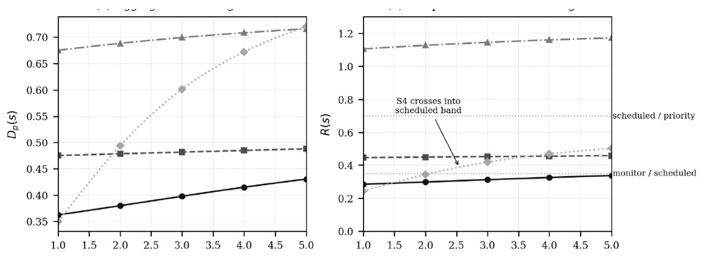
System S4 demonstrates the effect of the compensability exponent. Its profile is three healthy dimensions and one severe one. Table 8 shows its disposition across p.
Under arithmetic aggregation the near-total failure of S4’s batch interface is diluted by its otherwise clean profile and the system is dismissed. At p = 3 it enters the scheduled band. Since the analyst’s choice of p changes the governance outcome, that choice must be published rather than embedded in a tool. This is the concrete case for the reporting requirement in Section 4.8.
Figure 4 generalizes the point across the whole portfolio. The three systems with relatively even dimension profiles are almost flat in p, so for them the choice of exponent is immaterial. S4 rises steeply, overtaking S1 and S2 in panel (a) and crossing the monitor/scheduled edge in panel (b). Compensability therefore matters precisely for the systems that a weighted average handles worst, which is the class of system the exponent exists to protect against.
5.2. What κ and Γ Add: A Worked Ranking Case
The S1/S3 inversion in Table 7 already exists in D₂ alone, so it does not show what the attenuation and criticality terms add. The following worked case does. It is an illustrative case, labeled as such, using the manuscript’s own aggregation form R = D × κ × Γ, where D is the dimension aggregate, κ the change-activity attenuation, and Γ the criticality multiplier. Consider two illustrative systems with different change activity and criticality: System A has D = 0.70, is frozen (ĉ low, so κ = κ_min = 0.40) and is non-critical (Γ = 1.0), giving R_A = 0.70 × 0.40 × 1.0 = 0.28; System B has D = 0.50, is actively changing (κ = 1.0) and is critical (Γ = 1.4, two criticality features at the 0.2 step), giving R_B = 0.50 × 1.0 × 1.4 = 0.70. On D alone, A ranks above B (0.70 > 0.50); on R, B ranks above A (0.70 > 0.28). The headline ranking therefore changes because of κ and Γ, not because of D. The limits of this case are stated plainly: it is constructed to show the mechanism, it is not evidence that κ and Γ improve real decisions, and the sensitivity analysis in Section 5.3 shows that such flips are themselves sensitive to the parameter values.
Table 8: Sensitivity of System S4 to the Compensability Exponent Click to enlarge
| p | D (S4) | R (S4) | Band |
|---|---|---|---|
| 1 (arithmetic mean) | 0.350 | 0.244 | Monitor |
| 1.5 | 0.424 | 0.295 | Monitor |
| 2 (recommended) | 0.494 | 0.344 | Monitor |
| 3 | 0.601 | 0.419 | Scheduled |
Table 8: Sensitivity of System S4 to the Compensability Exponent
| p | D (S4) | R (S4) | Band |
|---|---|---|---|
| 1 (arithmetic mean) | 0.350 | 0.244 | Monitor |
| 1.5 | 0.424 | 0.295 | Monitor |
| 2 (recommended) | 0.494 | 0.344 | Monitor |
| 3 | 0.601 | 0.419 | Scheduled |
5.3. Full Sensitivity Analysis (Recomputed)
The sensitivity analysis required by Section 4.8 was recomputed from equations (2)–(5) and the stipulated inputs of Table 6. No new data were introduced. Table 9 varies the exponent p; Table 10 varies κ_min and the criticality step; the band edges are varied in the text following the table; Table 11 varies the weights.
On p alone, the numbers are as follows: at p = 1, S4 (0.244) is below S1 (0.284); at p = 2, S4 (0.344) is above S1 (0.298). The S1/S4 ranking does not survive variation in p. Applying the Section 4.8 rule, the S1/S4 ranking is therefore withdrawn as a finding: it must not be reported as a result, and the example is retained only to demonstrate the computation. The S3 ranking is robust to p, and the S2 ranking is second in every row of Table 9.
Varying κ_min moves R for frozen systems most (S1 rises from 0.091 at κ_min = 0.0 to 0.401 at κ_min = 0.6) and varying the criticality step moves R for critical systems most (S3 rises from 0.877 at step 0.1 to 1.378 at step 0.3), as expected; neither variation changes the ordering. Shifting the band edges by ±10% (0.315/0.63 and 0.385/0.77) leaves the ordering unchanged, but it does change a band assignment: at the lower edges (0.315/0.63), S4 moves from Monitor to Scheduled. Band assignments for systems near an edge are therefore not robust and must be reported with the band edges used. Gate assignments are unaffected by the band edges, because gates are evaluated independently of R.
Across the 1,000 Dirichlet draws over the weight simplex, S3 ranks first in 100% of draws (mean rank 1.00), S2 has mean rank 2.20 and is never last, S4 has mean rank 3.27 and is last in 47.5% of draws, and S1 has mean rank 3.52 and is last in 52.5% of draws. The S3 ranking is therefore robust to the weights; the S1/S4 and S2/S4 orderings are not. When the batch/integration dimension dominates the weights, S4 rises above S2 (R = 0.556 against 0.406). Any reported ranking must state the weights used and the result of this analysis, as Section 4.8 requires.
5.4. Unassessed Bounds: A Worked Example
Section 4.7 requires that a system with one missing dimension be reported as a range. Table 12 applies that rule to the illustrative portfolio, taking each system’s highest dimension as the missing one and computing the best case (missing dimension = 0) and worst case (missing dimension = 1) with equal weights and p = 2. The width of the range is the amount of information the missing dimension carries: for S4, whose batch/integration score (0.95) dominates its profile, the range is 0.094–0.360 (width 0.266), which crosses the Monitor/Scheduled band edge — the system cannot be banded at all until that dimension is measured. Systems with two or more missing dimensions are Unassessed and are not ranked.
Table 9: Sensitivity to the Compensability Exponent p (Equal Weights, κ_min = 0.4, Step 0.2) Click to enlarge
| p | R (S1) | R (S2) | R (S3) | R (S4) | Ordering (highest to lowest) |
|---|---|---|---|---|---|
| 1 | 0.284 | 0.446 | 1.106 | 0.244 | S3, S2, S1, S4 |
| 1.5 | 0.291 | 0.447 | 1.117 | 0.295 | S3, S2, S4, S1 |
| 2 | 0.298 | 0.449 | 1.127 | 0.344 | S3, S2, S4, S1 |
| 3 | 0.312 | 0.452 | 1.145 | 0.419 | S3, S2, S4, S1 |
Table 9: Sensitivity to the Compensability Exponent p (Equal Weights, κ_min = 0.4, Step 0.2)
| p | R (S1) | R (S2) | R (S3) | R (S4) | Ordering (highest to lowest) |
|---|---|---|---|---|---|
| 1 | 0.284 | 0.446 | 1.106 | 0.244 | S3, S2, S1, S4 |
| 1.5 | 0.291 | 0.447 | 1.117 | 0.295 | S3, S2, S4, S1 |
| 2 | 0.298 | 0.449 | 1.127 | 0.344 | S3, S2, S4, S1 |
| 3 | 0.312 | 0.452 | 1.145 | 0.419 | S3, S2, S4, S1 |
Table 10: Sensitivity to κ_min and Criticality Step (p = 2, Equal Weights) Click to enlarge
| Variation | R (S1) | R (S2) | R (S3) | R (S4) | Ordering |
|---|---|---|---|---|---|
| κ_min = 0.0 | 0.091 | 0.301 | 1.053 | 0.178 | S3, S2, S4, S1 |
| κ_min = 0.2 | 0.195 | 0.375 | 1.090 | 0.261 | S3, S2, S4, S1 |
| κ_min = 0.4 (baseline) | 0.298 | 0.449 | 1.127 | 0.344 | S3, S2, S4, S1 |
| κ_min = 0.6 | 0.401 | 0.522 | 1.165 | 0.427 | S3, S2, S4, S1 |
| Criticality step 0.1 | 0.242 | 0.385 | 0.877 | 0.315 | S3, S2, S4, S1 |
| Criticality step 0.2 (baseline) | 0.298 | 0.449 | 1.127 | 0.344 | S3, S2, S4, S1 |
| Criticality step 0.3 | 0.354 | 0.513 | 1.378 | 0.372 | S3, S2, S4, S1 |
Table 10: Sensitivity to κ_min and Criticality Step (p = 2, Equal Weights)
| Variation | R (S1) | R (S2) | R (S3) | R (S4) | Ordering |
|---|---|---|---|---|---|
| κ_min = 0.0 | 0.091 | 0.301 | 1.053 | 0.178 | S3, S2, S4, S1 |
| κ_min = 0.2 | 0.195 | 0.375 | 1.090 | 0.261 | S3, S2, S4, S1 |
| κ_min = 0.4 (baseline) | 0.298 | 0.449 | 1.127 | 0.344 | S3, S2, S4, S1 |
| κ_min = 0.6 | 0.401 | 0.522 | 1.165 | 0.427 | S3, S2, S4, S1 |
| Criticality step 0.1 | 0.242 | 0.385 | 0.877 | 0.315 | S3, S2, S4, S1 |
| Criticality step 0.2 (baseline) | 0.298 | 0.449 | 1.127 | 0.344 | S3, S2, S4, S1 |
| Criticality step 0.3 | 0.354 | 0.513 | 1.378 | 0.372 | S3, S2, S4, S1 |
Table 11: Sensitivity to the Weights (p = 2, κ_min = 0.4, Step 0.2) Click to enlarge
| Weights | R (S1) | R (S2) | R (S3) | R (S4) | Ordering |
|---|---|---|---|---|---|
| Equal (0.25 each, baseline) | 0.298 | 0.449 | 1.127 | 0.344 | S3, S2, S4, S1 |
| IF-dominant (0.7, 0.1, 0.1, 0.1) | 0.284 | 0.461 | 1.139 | 0.232 | S3, S2, S1, S4 |
| DG-dominant (0.1, 0.7, 0.1, 0.1) | 0.383 | 0.433 | 1.189 | 0.243 | S3, S2, S1, S4 |
| DR-dominant (0.1, 0.1, 0.7, 0.1) | 0.262 | 0.490 | 0.913 | 0.224 | S3, S2, S1, S4 |
| BIF-dominant (0.1, 0.1, 0.1, 0.7) | 0.242 | 0.406 | 1.240 | 0.556 | S3, S4, S2, S1 |
| Dirichlet simplex, 1,000 draws: most common orderings | — | — | — | — | S3, S2, S1, S4 (47.5%); S3, S2, S4, S1 (32.1%); S3, S4, S2, S1 (20.4%) |
Table 11: Sensitivity to the Weights (p = 2, κ_min = 0.4, Step 0.2)
| Weights | R (S1) | R (S2) | R (S3) | R (S4) | Ordering |
|---|---|---|---|---|---|
| Equal (0.25 each, baseline) | 0.298 | 0.449 | 1.127 | 0.344 | S3, S2, S4, S1 |
| IF-dominant (0.7, 0.1, 0.1, 0.1) | 0.284 | 0.461 | 1.139 | 0.232 | S3, S2, S1, S4 |
| DG-dominant (0.1, 0.7, 0.1, 0.1) | 0.383 | 0.433 | 1.189 | 0.243 | S3, S2, S1, S4 |
| DR-dominant (0.1, 0.1, 0.7, 0.1) | 0.262 | 0.490 | 0.913 | 0.224 | S3, S2, S1, S4 |
| BIF-dominant (0.1, 0.1, 0.1, 0.7) | 0.242 | 0.406 | 1.240 | 0.556 | S3, S4, S2, S1 |
| Dirichlet simplex, 1,000 draws: most common orderings | — | — | — | — | S3, S2, S1, S4 (47.5%); S3, S2, S4, S1 (32.1%); S3, S4, S2, S1 (20.4%) |
Table 12: Best/Worst-Case Ranges with One Dimension Missing (Equal Weights, p = 2) Click to enlarge
| System | Missing dimension | Best case (0) | Worst case (1) | Range width |
|---|---|---|---|---|
| S1 Eligibility | DG (0.55) | 0.206 | 0.443 | 0.237 |
| S2 Case management | DR (0.55) | 0.367 | 0.596 | 0.229 |
| S3 Payments | BIF (0.80) | 0.917 | 1.230 | 0.313 |
| S4 Correspondence | BIF (0.95) | 0.094 | 0.360 | 0.266 |
Table 12: Best/Worst-Case Ranges with One Dimension Missing (Equal Weights, p = 2)
| System | Missing dimension | Best case (0) | Worst case (1) | Range width |
|---|---|---|---|---|
| S1 Eligibility | DG (0.55) | 0.206 | 0.443 | 0.237 |
| S2 Case management | DR (0.55) | 0.367 | 0.596 | 0.229 |
| S3 Payments | BIF (0.80) | 0.917 | 1.230 | 0.313 |
| S4 Correspondence | BIF (0.95) | 0.094 | 0.360 | 0.266 |
5.5. Gates in the Illustrative Portfolio
Finally, S1 shows why the index cannot be used on its own. Although its R value of 0.298 places it in the monitor band, gate G1 is raised, which is the most time-critical information about this particular portfolio: the end of the vendor’s support period is an external date certain and does not wait for a fiscal cycle. Thus, a single number would put this portfolio at the bottom of the dashboard and be wrong in a way that a vector of scores, multipliers, and gates would not. G1 is raised for S1 because its COBOL platform is past vendor end-of-support (Table 5); it is not raised because of S1’s documentation-gap score.
6. Discussion
6.1. Report the Vector, Not the Scalar
The motivating problem is that executives receive no comparable signal, and the natural response thereto, production of a scalar, would reintroduce the failure under another name. In the example there are two ways in which a scalar value can be misleading: categories rather than bands (gates), and multiple dimensions collapsing onto one (profile). This is why Figure 1 produces a tuple, and why Figure 2 computes R before the gates are applied and then lets a raised gate escalate the system regardless of its band. I therefore propose that CTDI be reported as the tuple of the four normalized dimensions, κ, Γ, R, the gate flags, and the coverage status. R orders a queue, it does not explain it, and it should never be the sole item on a dashboard.
6.2. Strategic Reporting
In a multi-vendor estate the entity best positioned to provide the input data is often the entity that the score is meant to govern. Once this starts to affect funding, DR7 becomes acute [30]. Three options exist, none of them ideal. Input definitions can be tied to system-of-record extractions scheduler logs, incident systems, interface registers rather than to vendor attestations, with inevitably reduced dimensional coverage and hence higher Unassessed category values. Second, independent sporadic audits can be performed, validating a subset of reported values on a cyclical basis. Most crucially, CTDI should be decoupled by policy from any vendor payment, penalty or scorecard mechanism; the moment it becomes a lever for financial benefit or harm to the vendor, it ceases to be an indicator of candor, becoming instead a signal about reporting behaviors. Leaving it in the sphere of internal remedy sequence analysis preserves whatever integrity there is in the system.
Documentation-gap realization has challenges, not least because it is the only construct where human judgments are not directly mechanized, making it both the most prone to gaming and the one where practitioners report the most value [23]. It is consequently the most likely source of both new signals and of obfuscation.
6.3. Correlation and Portfolio-Level Risk
CTDI scores systems serially and the portfolio view is simply a listing of individually scored systems. Real estates violate independence because individual systems share integration middleware and database platforms, vendors, and the small pool of engineers with legacy institutional knowledge. A single common-mode failure threatens the entire portfolio, and summing or ranking independent probabilities fails to capture the increased risk. Modeling the dependencies in a portfolio is a natural extension of this work but falls outside the scope of this paper. Within a system, the correlation between interface fragility and batch/integration failure is addressed in Section 4.11.
6.4. Distributional Consequences
A remediation-sequencing instrument in human services determines who gets benefits infrastructure repaired, and this has consequences beyond the efficiency of the repair process. Three aspects of this are worth noting.
Firstly, measurement coverage is not distributed evenly, with systems serving smaller, rural, non-English-speaking, or other marginalized communities being more likely to be legacy systems on local platforms, poorly instrumented, and hence Unassessed. The rule in Section 4.7 that Unassessed equals more critical is there to prevent the reverse of what is intended, but a rule is not a certainty, and so an organization using CTDI should check, in practice, that systems serving particular communities are not consistently more likely to be Unassessed.
Secondly, criticality rubrics based on either volume or budget are intrinsically biased against low-volume services. The rubric in Section 4.5 solves this by prioritizing interruptions over absence of fallbacks, and harm over volume, since a system serving four thousand people without any manual fallback may well have higher harm per interruption than a system serving hundreds of thousands with a fully automated contingency process; an organization implementing a similar rubric should retain this property.
Lastly, debt is often inherited, and so the team maintaining a thirty-year-old eligibility system will have lower scores than their counterparts replacing it in-house, for no reason other than circumstance, possibly for years [26]. If and this is a large if CTDI scores are used for resource allocation, organizational transformation, or contract renegotiation, then the potential exists for the most critical systems to be penalized at the managerial level, undermining Section 6.2’s reliance on self-reporting for critical systems. There is nothing wrong with scoring the system and not the team, and with limiting the application of the rubric to remediation-sequencing purposes, however; those are the factors that make the construct work, and not a weakness.
6.5. Scope and Its Consequences
Section 1 states the scope limit: the four dimensions do not encompass all forms of technical debt. The consequences for decision-making are: (i) a low CTDI score does not mean a system has no technical debt — it means it has low measured exposure on these four dimensions; (ii) a system with high test or requirements debt could rank low and be under-prioritized if CTDI were used alone, so CTDI must be used alongside code-level (SQALE/CAST) and test-coverage evidence, not as a replacement; and (iii) the Unassessed rule (Section 4.7) means systems with missing data are not silently ranked low. The index is therefore presented as one governance input among several, not as a complete measure of technical debt.
6.6. From Ranking to Funding: Remediation Cost
A ranking by R alone cannot tell a board what to fund within a budget. For each system, the board needs the estimated remediation cost C and the expected risk reduction ΔR from a proposed intervention, and the decision-relevant quantity is ΔR/C — risk reduction per unit cost — not R alone. The manuscript now gives the worked form: rank candidate interventions by ΔR/C within the budget, subject to the hard gates, with C and ΔR estimated by the service owner and recorded alongside R. Where C is unknown, the ranking by R is a prioritization input only, not a funding decision. This is presented as an extension of the framework, with its own falsification condition in Section 8: that ΔR/C-ranked funding outperforms R-ranked funding on realized outcomes.
6.7. What CTDI Adds over Age and Change Activity
The simple baseline system age plus normalized change activity — can tell a board which systems are old and which are changing, but it cannot tell the board (i) which systems are fragile at their interfaces, (ii) which are failing in batch/integration, (iii) which have a documentation gap that makes replacement risky, or (iv) which systems should be escalated regardless of their score because a single dimension is severe (the hard gates). CTDI adds exactly those four pieces of information, in a single auditable tuple per system. The manuscript also states the limit: if the four dimensions add no out-of-sample predictive power over the baseline in the Section 8 study, that is a falsification of the index, and Section 8 now says so.
6.8. Practical Use
Data needed. For each system, the four dimension proxies (interface inventory and version/contract evidence; batch/integration failure rates from run logs; documentation coverage from a human-assessed inventory; and defect-recurrence rates from the incident system), change activity ĉ from version-control and deployment logs (not self-report — see Section 4.13), service criticality from the rubric (Table 4), and, for funding decisions, estimated remediation cost C and expected risk reduction ΔR (Section 6.6). Cadence. The index is calculated quarterly, aligned with the portfolio governance cycle, with gates re-checked on any material change (a failed batch run, a vendor-support withdrawal, or a security vulnerability); Unassessed systems are re-assessed at the next quarterly cycle. How results support decisions. Each quarterly governance pack contains (a) the ranked tuple list (R, gates, Unassessed status), (b) the best/worst-case ranges for systems with a missing dimension, (c) the Unassessed list as a priority assessment list, and (d) the ΔR/C ranking for candidate interventions within the available budget, subject to the gates. The pack does not, by itself, allocate the budget — that requires C and ΔR, as stated in Section 6.6.
7. Limitations and Threats to Validity
Construct validity. The four dimensions were selected for governance observability, not because evidence establishes them as the most predictive of modernization failure. That evidence is lacking, as the independent debt-identification approaches of Zazworka et al. demonstrate only modest concordance [21]; a composite of such indicators would inherit their weak interrelation. Interface fragility and batch/integration failure are plausibly correlated (Section 4.11); until the inter-dimension correlation is measured on a real portfolio, rankings driven mainly by those two dimensions should be treated as provisional, and the Section 8 protocol requires the correlation matrix and a re-estimation with correlated dimensions merged or down-weighted if any pair exceeds r = 0.70.
Internal validity. The dimensions are not unrelated, most notably interface fragility and batch failure rate, which are closely related concepts. Taken together, their equal inclusion in the metric overestimates their combined contribution to project risk, beyond their shared variance. An accurate assessment would require a multivariate analysis of the portfolio, which I have not performed [27].
Parameter arbitrariness. The values κ_min = 0.4, p = 2, the 0.2 criticality increment, and the band edges 0.35 and 0.70 are stipulated. The parameters are internally consistent, and their sensitivity is now established for p, κ_min, the criticality step, the band edges, and the weights (Section 5.3), but none are empirically grounded. The sensitivity analysis shows which conclusions depend on which stipulation; in particular, the S1/S4 ranking depends on p and the S4 band assignment depends on the band edges.
External validity. The illustration is hypothetical and was constructed by me to demonstrate the ranking inversion. This fact alone undermines any claim of external validity, as a fabricated example is not generalizable to actual portfolios. Even if it did not, Section 5 does not provide grounds for believing that the age heuristic is routinely reversed in practice.
7.0.1. Scope
Architectural debt, the category practitioners assess as most critical to address [22], is only indirectly captured by interface fragility and documentation gap. Requirements and test debt are not considered, and the cost of assessment is not modeled, which may be significant in a large portfolio.
8. A Validation Protocol for Future Work
Because the prioritization literature is characterized by proposals that were never empirically tested [13], I specify in advance what would falsify CTDI.
- Design. Retrospective cohort of at least thirty systems across at least three portfolios, with dimension inputs reconstructed from records as they stood at time t and outcomes observed over [t, t + 24 months].
- Outcome measures. Schedule variance against the baseline plan; cost variance; count of severity-1 and severity-2 production incidents; count of integration defects found after cutover; and occurrence of program re-baselining or cancellation.
- Baseline to beat. A two-variable model using system age and normalized change activity. This is the crucial term. Any composite can correlate with outcomes; CTDI earns its complexity only by explaining variance that age and change activity do not. If it fails to beat this baseline, the appropriate conclusion is that the two-variable model should be used instead, and that conclusion should be published. To isolate the contribution of the four dimensions, the comparison model adds the four dimensions to the baseline, so the incremental contribution is the difference in out-of-sample performance between the two models — change activity does not appear on both sides without attribution.
- Weight calibration. Fit weights on a training partition and evaluate on a held-out partition, reporting the degradation. Weights fitted and evaluated on the same data are not evidence.
- Gate evaluation. Test separately that gate-flagged systems did not have categorical failures of a certain type, since gates are a separate claim from the index and should be evaluated as such. Report the gate firing rate and the outcomes of gated versus non-gated systems, so that the gate thresholds can be calibrated.
- Pre-registration. Register thresholds, weights, and exponent before observing outcomes, as the construct offers ample freedom to fit a ranking after the fact.
Power. With n = 30 systems, the study is underpowered for small effects. For a correlation of r = 0.30 at α = 0.05 (two-sided), power is approximately 0.36, and for a medium effect (r = 0.50) it is approximately 0.81 (Fisher-z approximation). These are standard power calculations for a correlation, stated as such, and they are the reason the protocol now pre-specifies a minimum detectable effect and a target sample size for a follow-up study: n = 85 systems for 80% power at r = 0.30. I state plainly that n = 30 is small and that the first study is therefore a pilot.
8.0.1. Model comparison
The protocol pre-specifies the comparison criteria: out-of-sample R² (held-out weights, Section 4.10), AIC/BIC for the CTDI model against the baseline model, and a pre-registered primary outcome (24-month modernization/operational outcome, as in the original protocol). A further falsification condition is added: if the four dimensions add no out-of-sample predictive power over the baseline, the index is falsified; and if ΔR/C-ranked funding does not outperform R-ranked funding on realized outcomes, the funding extension in Section 6.6 is falsified.
8.0.2. Association, not causation
The outcomes are program-level, so the study tests association between CTDI scores and outcomes; it cannot show whether allocating funds by CTDI improves results. That would require a randomized or stepped-wedge allocation study, which is listed as future work, not claimed as part of this protocol. A dynamic extension — tracking R(s) across release cycles and vendor transitions to obtain leading rather than lagging signal — is attractive but should follow, not precede, cross-sectional validation. Governance boards meet on monthly and quarterly cycles while remediation moves these dimensions over quarters and years, so the reporting cadence of any operational deployment must be matched to the measurement’s actual response time, or the index will appear inert and be abandoned. A non-linear attenuation form (Section 4.13) is also listed as future work.
9. Conclusion
Technical debt measurement is well developed for engineering audiences and largely absent from the governance layer where modernization funding is decided. Reviewing four established quantification approaches against five governance-relevant attributes shows the gap is structural rather than incidental: these instruments were designed for a single system and a technical reader, and none specifies how its output should inform a funding or sequencing decision.
I have specified the Composite Technical Debt Index as a candidate bridge, precisely enough to be attacked: four governance-observable dimensions, threshold-anchored normalization, power-mean aggregation with an explicit compensability parameter, change-activity attenuation, separately reported service criticality, non-scored hard gates, and an explicit Unassessed status for systems that cannot be measured. A hypothetical portfolio illustrates how the construct is computed, that the choice of aggregation exponent can change a governance disposition — which is why that choice must be published rather than buried in tooling — and that some rankings in the illustration do not survive sensitivity analysis, which is why they are withdrawn rather than reported.
The construct is unsubstantiated, and I regard the validation process described in Section 8 as its better contribution than the index itself. Two conditions on its use are suggested by the analysis, not by prudence. The index should be reported as a vector with the gate flags and coverage indication, not as a scalar with the last system shown as most time-constrained. It should not be used for vendor payments and personnel evaluations because a measure based on contributions by the parties assessed will reflect their reporting practices, not their contribution. In the context of public sector human services, these are not merely administrative concerns: the instrument is an allocation mechanism for the repair of infrastructure essential to subsistence, and a methodological improvement that fails to account for the least quantified systems would be a worse guide to public investment than the narrative analysis it supplanted.
- U.S. Government Accountability Office, “Information technology: Agencies need to develop modernization plans for critical legacy systems,” Report GAO-19-471, Washington, DC, USA, June 2019.
- U.S. Government Accountability Office, “Information technology: Agencies need to plan for modernizing critical decades-old legacy systems,” Report GAO-25-107795, Washington, DC, USA, July 2025.
- W. Cunningham, “The WyCash portfolio management system,” in Addendum to the Proceedings on Object-Oriented Programming Systems, Languages, and Applications (OOPSLA ’92), 1992, pp. 29–30, doi: 10.1145/157709.157715.
- P. Kruchten, R. L. Nord, I. Ozkaya, “Technical debt: From metaphor to theory and practice,” IEEE Software, vol. 29, no. 6, pp. 18–21, 2012, doi: 10.1109/MS.2012.167.
- P. Avgeriou, P. Kruchten, I. Ozkaya, C. Seaman, “Managing technical debt in software engineering (Dagstuhl Seminar 16162),” Dagstuhl Reports, vol. 6, no. 4, pp. 110–138, 2016, doi: 10.4230/DagRep.6.4.110.
- Z. Li, P. Avgeriou, P. Liang, “A systematic mapping study on technical debt and its management,” Journal of Systems and Software, vol. 101, pp. 193–220, 2015, doi: 10.1016/j.jss.2014.12.027.
- R. Verdecchia, P. Kruchten, P. Lago, I. Malavolta, “Building and evaluating a theory of architectural technical debt in software-intensive systems,” Journal of Systems and Software, vol. 176, art. no. 110925, 2021, doi: 10.1016/j.jss.2021.110925.
- C. Seaman, Y. Guo, “Measuring and monitoring technical debt,” Advances in Computers, vol. 82, pp. 25–46, 2011, doi: 10.1016/B978-0-12-385512-1.00002-5.
- J.-L. Letouzey, “The SQALE method for evaluating technical debt,” in Proc. 3rd International Workshop on Managing Technical Debt (MTD), 2012, pp. 31–36, doi: 10.1109/MTD.2012.6225997.
- B. Curtis, J. Sappidi, A. Szynkarski, “Estimating the principal of an application’s technical debt,” IEEE Software, vol. 29, no. 6, pp. 34–42, 2012, doi: 10.1109/MS.2012.156.
- A. Nugroho, J. Visser, T. Kuipers, “An empirical model of technical debt and interest,” in Proc. 2nd Workshop on Managing Technical Debt (MTD), 2011, pp. 1–8, doi: 10.1145/1985362.1985364.
- T. Besker, A. Martini, J. Bosch, “Software developer productivity loss due to technical debt: A replication and extension study examining developers’ development work,” Journal of Systems and Software, vol. 156, pp. 41–61, 2019, doi: 10.1016/j.jss.2019.06.004.
- V. Lenarduzzi, T. Besker, D. Taibi, A. Martini, F. Arcelli Fontana, “A systematic literature review on technical debt prioritization: Strategies, processes, factors, and tools,” Journal of Systems and Software, vol. 171, art. no. 110827, 2021, doi: 10.1016/j.jss.2020.110827.
- C. Jaspan, C. Green, “Defining, measuring, and managing technical debt,” IEEE Software, vol. 40, no. 3, pp. 15–19, 2023, doi: 10.1109/MS.2023.3242137.
- B. Kitchenham, S. Charters, “Guidelines for performing systematic literature reviews in software engineering,” EBSE Technical Report EBSE-2007-01, Keele University and University of Durham, 2007.
- W. N. Behutiye, P. Rodríguez, M. Oivo, A. Tosun, “Analyzing the concept of technical debt in the context of agile software development: A systematic literature review,” Information and Software Technology, vol. 82, pp. 139–158, 2017, doi: 10.1016/j.infsof.2016.10.004.
- A. Ampatzoglou, A. Ampatzoglou, A. Chatzigeorgiou, P. Avgeriou, “The financial aspect of managing technical debt: A systematic literature review,” Information and Software Technology, vol. 64, pp. 52–73, 2015, doi: 10.1016/j.infsof.2015.04.001.
- A. Martini, J. Bosch, M. Chaudron, “Architecture technical debt: Understanding causes and a qualitative model,” in Proc. 40th Euromicro Conference on Software Engineering and Advanced Applications (SEAA), 2014, pp. 85–92, doi: 10.1109/SEAA.2014.65.
- R. L. Nord, I. Ozkaya, P. Kruchten, M. Gonzalez-Rojas, “In search of a metric for managing architectural technical debt,” in Proc. Joint Working IEEE/IFIP Conference on Software Architecture and European Conference on Software Architecture (WICSA/ECSA), 2012, pp. 91–100, doi: 10.1109/WICSA-ECSA.212.17.
- E. da S. Maldonado, E. Shihab, “Detecting and quantifying different types of self-admitted technical debt,” in Proc. 7th IEEE International Workshop on Managing Technical Debt (MTD), 2015, pp. 9–15, doi: 10.1109/MTD.2015.7332619.
- N. Zazworka, A. Vetrò, C. Izurieta, S. Wong, Y. Cai, C. Seaman, F. Shull, “Comparing four approaches for technical debt identification,” Software Quality Journal, vol. 22, no. 3, pp. 403–426, 2014, doi: 10.1007/s11219-013-9200-8.
- N. A. Ernst, S. Bellomo, I. Ozkaya, R. L. Nord, I. Gorton, “Measure it? Manage it? Ignore it? Software practitioners and technical debt,” in Proc. 10th Joint Meeting on Foundations of Software Engineering (ESEC/FSE), 2015, pp. 50–60, doi: 10.1145/2786805.2786848.
- N. Rios, R. O. Spínola, M. Mendonça, C. Seaman, “The most common causes and effects of technical debt: First results from a global family of industrial surveys,” in Proc. 12th ACM/IEEE International Symposium on Empirical Software Engineering and Measurement (ESEM), 2018, art. no. 39, pp. 1–10, doi: 10.1145/3239235.3268917.
- J. Holvitie, S. A. Licorish, R. O. Spínola, S. Hyrynsalmi, S. G. MacDonell, T. S. Mendes, J. Buchan, V. Leppänen, “Technical debt and agile software development practices and processes: An industry practitioner survey,” Information and Software Technology, vol. 96, pp. 141–160, 2018, doi: 10.1016/j.infsof.2017.11.015.
- P. Avgeriou, I. Ozkaya, A. Chatzigeorgiou, M. Ciolkowski, N. A. Ernst, R. J. Koontz, E. Poort, F. Shull, “Technical debt management: The road ahead for successful software delivery,” in Proc. IEEE/ACM International Conference on Software Engineering: Future of Software Engineering (ICSE-FoSE), 2023, pp. 15–30, doi: 10.1109/ICSE-FoSE59343.2023.00007.
- H. Ghanbari, S. Ahuja, B. Lee, J. Gaskin, “Who should pay for technical debt? Exploring software professionals’ perceptions about technical debt accountability,” Information and Organization, vol. 35, no. 3, art. no. 100589, 2025, doi: 10.1016/j.infoandorg.2025.100589.
- M. Nardo, M. Saisana, A. Saltelli, S. Tarantola, A. Hoffmann, E. Giovannini, Handbook on Constructing Composite Indicators: Methodology and User Guide. Paris, France: OECD Publishing, 2008, doi: 10.1787/9789264043466-en.
- G. Munda, Social Multi-Criteria Evaluation for a Sustainable Economy. Berlin, Germany: Springer, 2008, doi: 10.1007/978-3-540-73703-2.
- T. L. Saaty, The Analytic Hierarchy Process: Planning, Priority Setting, Resource Allocation. New York, NY, USA: McGraw-Hill, 1980.
- M. Strathern, “‘Improving ratings’: Audit in the British University system,” European Review, vol. 5, no. 3, pp. 305–321, 1997, doi: 10.1002/(SICI)1234-981X(199707)5:3<305::AID-EURO184>3.0.CO;2-4.
- M. I. Murillo, G. López, R. O. Spínola, J. Guzmán, N. Rios, A. Pacheco, “Identification and management of technical debt: A systematic mapping study update,” Journal of Software Engineering Research and Development, vol. 11, art. no. 8, 2023, doi: 10.5753/jserd.2023.2671.
- U. M. Graetsch, R. Hoda, H. Khalajzadeh, M. Shahin, J. Grundy, “Managing technical debt in a multidisciplinary data intensive software team: An observational case study,” Journal of Systems and Software, vol. 230, art. no. 112546, 2025, doi: 10.1016/j.jss.2025.112546.
- T. B. S. Gomes, D. A. de M. Loiola, A. R. Santos, “Technical debt tools: A survey and an empirical evaluation,” Journal of Software Engineering Research and Development, vol. 12, art. no. 8, 2024, doi: 10.5753/jserd.2024.3591.
- F. E. de O. Calixto, E. C. Araújo, E. L. G. Alves, “Technical debt in pull requests: Insights from Apache projects,” Journal of Software Engineering Research and Development, vol. 13, art. no. 12, 2025, doi: 10.5753/jserd.2025.5722.
- A. Melo, R. Fagundes, V. Lenarduzzi, W. B. Santos, “Identification and measurement of requirements technical debt in software development: A systematic literature review,” Journal of Systems and Software, vol. 194, art. no. 111483, 2022, doi: 10.1016/j.jss.2022.111483.
No related articles were found.