This paper outlines a method for obtaining the optimal control policy for an autonomous vehicle appro med that traffic signal phase and timing information can be made available to the autonomous vehicle as the vehicle approaches the traffic signal. Constraints on the vehicle’s speed and acceleration are considered and a microscopic fuel consumption model is considered. The objective is to minimize a weighted sum of the travel time and the fuel consumption. The problem is solved using the Deep Deterministic Policy Gradient algorithm under the reinforcement learning framework. First, the vehicle model, system constraints, and fuel consumption model are translated to the reinforcement learning framework, and the reward function is designed to guide the agent away from the system constraints and towards the optimum as defined by the objective function. The agent is then trained for different relative weights on the travel time and the fuel consumption, ults are presented. Several considerations for deploying such reinforcement learning-based ents are also discussed.

1. Introduction

Connected and autonomous vehicle (CAV) technology is increasingly being considered in research and development and is already being assimilated into real-world transport systems due to potential benefits in traffic throughput and energy consumption management [1, 2]. In connected vehicles (CVs), real-time information about the environment, including other road users and traffic signals is made avail- able to the vehicle’s operator through vehicle-to-vehicle (V2V) and vehicle-to-infrastructure (V2I) communication. Environment information may also be directly sensed, but can be limited to the immediate vicinity of vehicles and may require high processing power. In autonomous vehicles (AVs), the driver is not in the loop. Hence, there is a great chance of efficient use of shared or sensed information and the diminution of human errors.

In this paper, our focus is on the utilization of the re- inforcement learning (RL) framework for solving the eco- driving problem of an AV approaching a signalized inter- section. As a vehicle enters within some range of a traffic signal, using V2X communication, it receives the traffic signal phase and timing (SPaT) information. The vehicle then seeks to minimize energy consumption as it approaches the signalized intersection. As shown in literature, the eco- driving problem can be approximately solved by regulating advisory speed limits which, if followed, will minimize engine idle time as the vehicle approaches the traffic stop [3, 4, 5]. The problem can also be formulated as an optimal control problem that deals with finding a control policy to minimize a specified objective function [6, 7, 8].

Traditional methods for solving optimal control problems are based on the calculus of variations and the Pontryagin minimum principle to identify necessary conditions for optimal controls. Then, iterative numerical techniques are used to solve the two-point boundary-value problem to find the optimal controls [9]. In general, the eco-driving optimization problem is non-convex due to the nature of the traffic light constraints. Due to the complexity of fuel consumption models, the eco-driving optimization problem can be formulated to indirectly minimize the energy through other performance metrics, such as the acceleration [7]. In [10] it is shown that such alternatives may not yield a true energy optimum. Assuming the model of the problem is known, dynamic programming can also be used to simplify the problem into simpler, nested sub-problems, and then recursively solve the sub-problems [11, 12]. Generally, real-world vehicle systems are non-linear and highly complex. The RL framework provides a model-free approach to optimal control.

In RL, an agent interacts with its environment, observes the state of the environment, takes an action that may change the state, and observes the new state. Some supervisory signal is provided to the agent in the form of a reward to guide it towards the desired goal [13]. The agent exploits the knowledge from its exploration in making informed decisions. Using this framework, control policies with acceptable levels of optimality can be obtained even with system constraints, provided that a proper reward structure is designed. When the states of the system are not entirely known, or the representation of the states in a table is prohibitively cumbersome, a function approximator may further be employed to augment learning as the agent explores. Given a mapping of a set of inputs to some outputs, assuming that there is an unknown underlying function that consistently maps the inputs to outputs, a function approximator seeks to approximate this function. If the function to be estimated is continuous, the universal approximation theorem [14] provides a basis for the estimation of such a function using a weighted sum of non-linear functions. Artificial neural networks are a typical class of such a weighted sum. Thus, using a supervised-learning framework, the value function can be approximated. In traditional supervised machine learning, a neural network is presented with a data set and some supervisory labels to guide the learning process. In training, the neural network adjusts its weights based on the deviation of its prediction from the true value as measured by a loss function. The loss is regarded as a measure of how close the prediction is to the true value and is minimized by adjusting the weights in the network. This process continues until an acceptable set of weights is achieved [15]. When a machine learning network has multiple layers, it is referred to as a deep-learning network [16]. The fusion of deep learning and RL is generally referred to as deep RL [17] and has inspired many successful artificial intelligent systems [18].

In this paper, we consider a direct fuel minimization problem, and propose a deep RL framework for solving it. For the eco-driving problem, we are concerned with the vehicle energy optimization as it approaches a signalized intersection, given the traffic signal phase information. In contrast to existing works, we do not assume any structure of the solution, discretize the action set, or indirectly minimize the fuel consumption, but attempt to tackle the eco-driving problem without the aforementioned simplification [19, 20, 21]. In addition, only the current signal information is available and future SPaT is unknown to autonomous vehicles. The problem is solved based on deep neural networks in the RL framework.

2. Problem Formulation

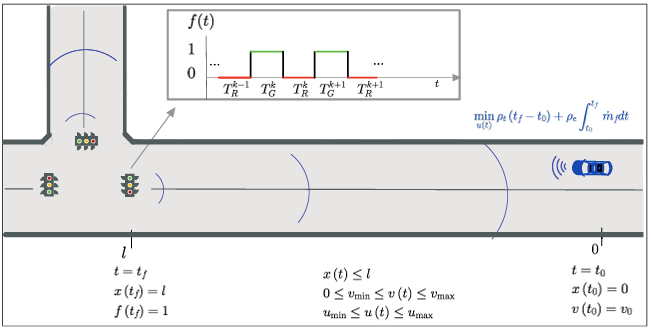
The task is to optimally control an autonomous vehicle approaching a signalized intersection. At time 𝑡₀, the vehicle starts at a point 𝑥₀ = 0 with an initial speed 𝑣₀. The traffic signal head is 𝑙 meters away from the vehicle. The eco-driving problem is illustrated in Fig. 1.

2.1. System Model

To simplify the model, let us approximate the vehicle by a unit point mass that can be accelerated by using the throttle or decelerated by using the brake. The dynamics of the vehicle are modeled by a double integrator given by

$$\begin{bmatrix} \dot{x}(t) \\ \dot{v}(t) \end{bmatrix} = \begin{bmatrix} 0 & 1 \\ 0 & 0 \end{bmatrix} \begin{bmatrix} x(t) \\ v(t) \end{bmatrix} + \begin{bmatrix} 0 \\ 1 \end{bmatrix} u(t)\tag{1}$$

where 𝑥(𝑡) and 𝑣(𝑡) are the position and velocity, respectively.

2.2. Constraints

The next step is to define the physical constraints on the state and control values. For the state constraints, if 𝑡₀ is the starting time, and 𝑡 _𝑓 is the time of arrival at the traffic signal head, then clearly, 

$$\left[\begin{array}{c} x(t_0) \\ v(t_0) \end{array}\right] = \left[\begin{array}{c} 0 \\ v_0 \end{array}\right],\tag{2}$$

and

𝑥(𝑡 _𝑓 ) = 𝑙.                                            (3)

If we assume that the vehicle does not back up, then additional constraints

0 ≤ 𝑥(𝑡) ≤ 𝑙,

0 ≤ 𝑣_min ≤ 𝑣(𝑡) ≤ 𝑣_max

are also imposed, where 𝑣_max is the road speed limit or the physical velocity constraint of the vehicle. With 𝑣_min, the vehicle can be constrained not to come to a full stop, and can be adjusted to decrease queue-length build-up. The acceleration is constrained by the engine capacity of the vehicle, and the maximum deceleration is limited by the braking system parameters. If the maximum acceleration is 𝑢_max > 0 and the maximum deceleration is 

𝑢_min < 0,

then the controls must satisfy

𝑢_min ≤ 𝑢(𝑡) ≤ 𝑢_max.                                     (4)

The traffic light signal at the intersection switches between the green light and the red light consecutively, and is repre- sented by a rectangular pulse signal

$$f(t) = \begin{cases} 1 & \text{for } t \in T_G \\ 0 & \text{for } t \in T_R \end{cases} \tag{5}$$

where 𝑇_𝐺 are 𝑇_𝑅 are the time intervals in which the traffic signal is green and red, respectively. The vehicle can only cross the intersection during the green interval, that is, 𝑡 _𝑓 ∈ 𝑇_𝐺.

2.3. Objective function

The objective function to be minimized includes a term for the duration of travel and a fuel consumption term. The following fuel consumption model is derived from the estimation in [22], with an additional assumption of fuel consumption during deceleration:

$$\dot{m}_f = \begin{cases} m_\alpha + m_\beta u(t), & u(t) \geq 0, \\ \alpha_0, & u(t) < 0, \end{cases} \tag{6}$$

where

$$m_\alpha = \alpha_0 + \alpha_1 v(t) + \alpha_2 v(t)^2 + \alpha_3 v(t)^3 \tag{7}$$

$$\\ m_\beta = \beta_0 + \beta_1 v(t) + \beta_2 v(t)^2 \tag{8}$$

and 𝛼₀, 𝛼₁, 𝛼₂, 𝛼₃,𝛽₀, 𝛽₁ and 𝛽₂, are approximated through a curve fitting process. The performance measure is given by

$$J = \min_{u(t)} \rho_t (t_f – t_0) + \rho_e \int_{t_0}^{t_f} \dot{m}_f \, dt \tag{9}$$

where 𝜌_𝑡 and 𝜌_𝑒 are two weight parameters. When 𝜌_𝑒 = 0, it is a minimum time problem; when 𝜌_𝑡 = 0, it is a minimum energy problem.

3. Reinforcement Learning Approach

3.1. Brief Review of Reinforcement Learning

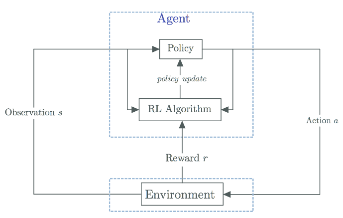
The schematic of the RL framework is depicted in Fig. 2. RL involves the interaction between an agent and environment. At each time step, the agent observes some state, 𝑠 of the environment from the set of states 𝒮, and on that basis selects an action, 𝑎 from the set of actions 𝒜, according to a policy 𝜋(𝑠). After one step, in part as a consequence of performing its action, the environment transitions to a new state, 𝑠^′. The action also fetches the agent an immediate reward, 𝑟(𝑠, 𝑎) from the set of rewards ℛ.

The action-value function or 𝑄-value function 𝒬(𝑠, 𝑎) maps each state-action pair to a value that represents the expected total long-term reward starting from the given state 𝑠, taking action 𝑎, and following the policy 𝜋(𝑠) onwards. The 𝑄-learning algorithm is a value-based RL algorithm that tries to learn the 𝑄-value function [23]. For any given state 𝑠 observed by a 𝑄-learner, the policy 𝜋(𝑠) selects the action that maximizes the action-value function 𝒬(𝑠, 𝑎):

$$\pi(s) = \arg\max_{a} Q(s,a).$$

The 𝑄-vlaue function is mostly estimated using the recursive Bellman equation [24]

$$Q(s,a) \leftarrow (1 – \eta) Q(s,a) + \eta \left( r(s,a) + \gamma \left[ \max_{a’} Q(s’, a’) \right] \right).$$

The learning rate 𝜂 determines to what extent the new information overrides the old while the discount factor 𝛾 helps to discount the future rewards in the current consideration. The deep 𝑄-network (DQN) learner is a 𝑄-learner with a function approximator– 𝒬(𝑠, 𝑎|𝜙), parameterized by 𝜙.DQN is applicable to environments with continuous states, but the action set is discrete. For stable training, a set of previous experiences, 𝑒 = (𝑠, 𝑎,𝑟, 𝑠′) is sampled from an experience replay buffer of size 𝒟 according to a specified minibatch size ℬ and fed into the neural network [25]. The DQN-learner has its number of inputs and outputs equal to the size of the state vector and discrete action space, respectively. Because every training step updates the weights, and by extension, the 𝑄-values of entire state-action pairs, a target network is created to keep the weights constant until after 𝑛𝜏 steps. Let the target network be parameterized by 𝜙𝑡. The target network is updated according to

𝜙𝑡 ←𝜏𝜙+(1−𝜏)𝜙t

for some 𝜏 ≪ 1 [26].

When the number of possible actions is infinitely large, such as in continuous action space, it becomes difficult to calculate the 𝑄-values for actions and compare all of them. It is also computationally intensive to solve max_𝑎 𝒬(𝑠, 𝑎) at every decision step. The Deep Deterministic Policy Gradient (DDPG) approach was introduced to solve this problem and extend 𝑄-learning to environments with continuous action spaces [26]. DDPG combines both deep 𝑄-learning and deep policy gradients (PG) approaches by concurrently learning a 𝑄-function and a policy. The PG approach to RL was originally proposed in [24] to handle discontinuities in the value function approximation that impact convergence assurances. The deep PG method aims to model and optimize the policy 𝜋(𝑠 |𝜃) directly using an actor-critic model: the critic updates the value function parameters 𝜙 for 𝒬(𝑠, 𝑎 |𝜙) and the actor updates the policy parameters 𝜃 for 𝜋(𝑠 |𝜃), guided by the critic. As with critic networks, an actor target network – 𝜋(𝑠 |𝜃_𝑡 ), parameterized by 𝜃_𝑡 – is also employed to ensure the stability of the optimization. DDPG models the policy as a deterministic decision 𝜇(𝑠 |𝜃), rather than a probability distribution over actions 𝜋(𝑠 |𝜃) [27].

The critic network has an input layer size equal to the addition of the sizes of the observation vector and the action, and a single output to represent the action-value function mapping. The actor network has an input layer size equal to the size of the observation vector 𝑠, and an output layer equal to the size of the action to represent the policy [17]. Mini-batch sampling from experience replay buffer and soft target updates are also extended to the actor network. Being an off-policy approach, DDPG does not require full trajectories and can generate samples by following a behavior policy different from the target policy 𝜇(𝑠 |𝜃). Noise 𝒵 is added to actions for expansive exploration during training, with variance 𝜎² and variance decay 𝜍² . The noise added is typically uncorrelated, and zero-mean Gaussian.

3.2. Reinforcement Learning Approach to Eco-driving Problems

To implement RL algorithms in a digital computer numerically, the system differential equation must be discretized. The acceleration 𝑢(𝑡) is generated by a digital computer followed by a zero-order holder (ZOH), then 𝑢(𝑡) will be piece-wise constant. Let ℎ be a very small sampling period, and 

𝑢(𝑡)=𝑢(𝑛ℎ)≜𝑎(𝑛)

for 𝑛ℎ ≤ 𝑡 < (𝑛 + 1)ℎ. The acceleration changes values only at discrete-time instants. For this input, where

𝜉(𝑛)=𝑥(𝑛ℎ)

and

𝜈(𝑛)=𝑣(𝑛ℎ),

the discrete-time model becomes

$$\begin{bmatrix} \xi(n+1) \\ v(n+1) \end{bmatrix} = \begin{bmatrix} 1 & h \\ 0 & 1 \end{bmatrix} \begin{bmatrix} \xi(n) \\ v(n) \end{bmatrix} + \begin{bmatrix} \frac{h^2}{2} \\ h \end{bmatrix} a(n).$$

In the following paragraphs, we will define the sets of states, actions, and rewards (𝒮,𝒜andℛ).

3.2.1. State Set 𝒮

The agent is placed in the vehicle. The agent observes the traffic signal, 𝑓 (𝑡), the position 𝑥(𝑡) and the velocity 𝑣(𝑡) at each sampling instance 𝑛ℎ. The observation vector at the time instant 𝑡 = 𝑛ℎ is thus the augmented state vector

$$s_n = \left[ \xi(n)\ \ v(n)\ \ f(nh)\ \ n \right]^T \in \mathcal{S} \tag{10}$$

that includes the traffic signal and the instant at which the traffic signal is observed, and 𝒮 is the set of all states. The initial state is [ 0 𝜈(0) 𝑓 (0) 0 ]^𝑇 . A state 𝑠_𝑛 is a terminal state whenever 𝜈(𝑛) ≤ 𝑣_min, or 𝜈(𝑛) ≥ 𝑣_max, or 

𝜉(𝑛)≥𝑙.

We let 𝒮_𝑇 ⊂ 𝒮 denote the set of terminal states. After a terminal state, the agent resets to the initial state

3.2.2. Action Set 𝒜

It is assumed that the admissible acceleration at any step, 𝑎(𝑛), is constrained to a closed interval

𝒜 = [𝑢_min 𝑢_max].          (11)

At each time instant 𝑛ℎ, the agent selects an action

𝑎(𝑛) = 𝜇(𝑠_𝑛 |𝜃) ∈ 𝒜.

The goal is to find the optimal 𝜇^∗(𝑠_𝑛 |𝜃) at each instant 𝑛 based on the environment state 𝑠_𝑛 .

3.2.3. Reward Set ℛ

To design the reward system to minimize time and fuel consumption, events of success and failure are defined. In the context of the problem, success is only achieved by the agent once it crosses the traffic signal within the green time interval and all constraints are satisfied from the beginning to the end. Failure occurs when the system constraints are violated. Once success or failure is encountered, the state is a terminal state and exploration stops. For the eco-driving problem formulated in Section 2, the long-term reward can be expressed as 

$$J_r = -\sum_{n=0}^{N} \left[ \rho_t h + \rho_e h M_n \right]$$

where 𝑁 is such that 𝑠_𝑁 ∈ 𝒮_𝑇 and

$$M_n = \frac{1}{h} \int_{nh}^{(n+1)h} \dot{m}_f \, dt$$

The term

$$M_n = \alpha_0 + \max\left\{ \operatorname{sgn}(a(n)), 0 \right\}$$

$$\left( \alpha_1 \psi_1 + \alpha_2 \psi_2 + \alpha_3 \psi_3 + (\beta_0 + \beta_1 \psi_1 + \beta_2 \psi_2) a(n) \right)$$

where

$$\psi_1(v(n),a(n),h) = v(n) + \frac{a(n)h}{2},$$

$$\quad \psi_2(v(n),a(n),h) = v(n)^2 + v(n)a(n) + \frac{a(n)^2 h^2}{3},$$

$$\quad \psi_3(v(n),a(n),h) = v(n)^3 + v(n)a(n)^2 h^2 + \frac{3v(n)^2 a(n) h}{2} + \frac{a(n)^3 h^3}{4}.$$

The reward function has three components:

𝑅(𝑛)=𝑟1(𝑛)+𝑟2(𝑛)+𝑟3(𝑛)

where

$$r_1(n) = -\rho_t h – \rho_e h M_n,$$

$$\quad r_2(n) = \begin{cases} 0 & \text{if } v_{\min} \leq v(n) \leq v_{\max}, \\ -p_2 & \text{otherwise}, \end{cases}$$

$$\quad r_3(n) = \begin{cases} -p_3 & \text{if } f(N) = 0, \\ 0 & \text{otherwise}. \end{cases}$$

The first component is related to the objective function. If all constraints are satisfied from the beginning to the end,

𝑅(𝑛) = 𝐽_𝑟 . The second component is related to the velocity constraint. If it is violated, a penalty 𝑝₂ > 0 is given. The third constant is related to the traffic signal constraint. If it is violated, a large penalty 𝑝₃ > 0 is given. The actions leading to constraint violations are thus discouraged. To guide the agent to a true optimum, and avoid getting stuck in local optima when the state constraints are violated, we ensure −𝑝₂ ≪ −𝑝₃ ≪ 𝐽_𝑟 . The discrete reward signals help avoid undesirable states, while the continuous reward signal provides a smooth manifold for improving convergence.

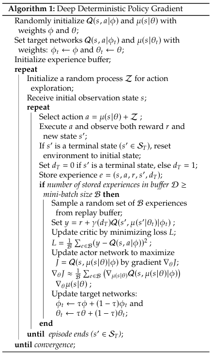
4. DDPG Algorithm

The algorithm applied here is based on the DDPG algorithm. We refer the interested reader to [26] for a comprehensive explanation of the DDPG algorithm. The pseudo-code applied to solve the eco-driving problem is outlined in Algorithm 1.

5. Simulation

The eco-driving problem is simulated using the parameters in the following sub-sections.

5.1. Agent environment parameters

For simulation, the upper limit of the distance observation is chosen as

0 ≤ 𝜉(𝑛) ≤ 𝑙 + Δ

where Δ = ℎ𝑣_max so that for a sampled distance very close to 𝑙, a maximum acceleration input is still admissible. The traffic signal for training the agent is delayed by a time-gap of 𝑡_𝑔 seconds so that there is a buffer time between the start of the green time interval and when the vehicle will cross the intersection after training. A high number of training samples has been found to improve the learning processes where the reward function is discontinuous [28]. Hence the mini-batch size is chosen to be 120. All other parameters of the agent are chosen as shown in Table 1. The fuel consumption model coefficients are borrowed from the fuel consumption model used in [22].

5.2. Neural Network Parameters

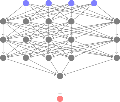
The actor and critic neural network parameters are shown in Fig. 3 and Fig. 4 respectively. The actor neural network is composed of an input layer with four inputs and three fully connected (FC) layers, each of 48 neurons with recti- fied linear unit (ReLU) activation. An FC layer consisting of a single neuron with a tanh function activation follows sequentially, and the result is passed to a scaling layer with a bias of −0.5 and a scaling factor of 2.5 for the resulting output layer.

The critic neural network gets inputs from both observa- tion and action and concatenates them. Before concatena- tion, the observation is passed through a 48 neuron ReLU FC layer and a 48 neuron FC layer, while the action is passed through a 48 neuron FC layer. The concatenation is an element-wise addition of the two 48 × 1 resulting vectors, and its output is fed through a 48 neuron RELU FC layer to the network output, a single neuron FC layer. The results of the simulation are presented next.

𝑠_𝑛 (1) 𝑠_𝑛 (2) 𝑠_𝑛 (3) 𝑠_𝑛 (4)

𝑠_𝑛 (1) 𝑠_𝑛 (2) 𝑠_𝑛 (3) 𝑠_𝑛 (4)   𝑎_𝑛

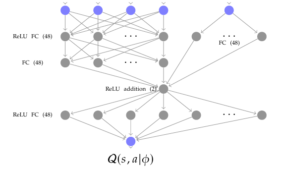
Table 1: Training parameters for eco-driving with reinforcement learning

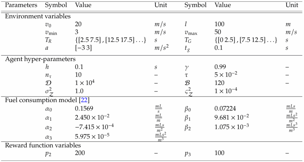
Table 2: Training results for different DDPG-based eco-driving cases

5.3. Results

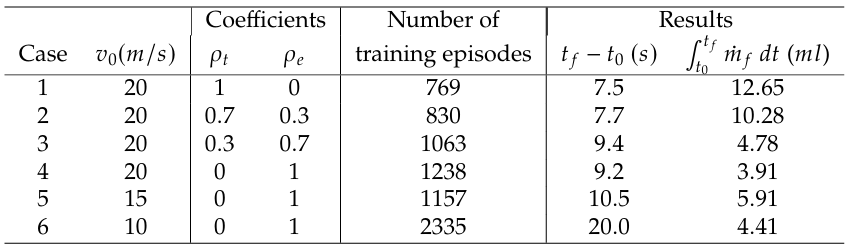
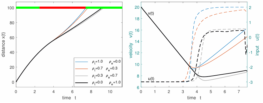
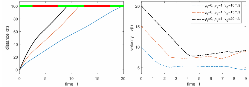
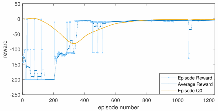
The agent is trained for the cases listed in Table 2. In gen- eral, there is no guarantee that the agent will achieve an optimal solution. The training is stopped when the moving average of the reward plateaus and the difference between the critic’s estimate (Episode 𝑄₀) and the moving average of the reward is small. Episode 𝑄₀ is the expected long- term reward estimated by the critic at the beginning of each episode, given an initial environment observation. It provides a measure of how well the critic has learned the environment. The moving average reward considered is based on the previous 10 episode rewards. After training for the number of episodes as listed in the table, the agent is simulated in the same environment from the initial state and the distance of the vehicle to the traffic signal against time is shown in Fig. 5. The velocity and input plots for the first 7.5 seconds are also shown in Fig. 5 for cases 1 − 4 in Table 2. In each of these cases, the agent decelerates the vehicle for some time and then accelerates almost sharply to save time. Deceleration sacrifices previous kinetic energy, hence, the agent does not consider conserving the energy it had at the start. An approach to check this behavior is to formulate a multi-stage energy minimization problem over multiple signal stops so that the vehicle considers economizing its energy throughout the journey. Increasing the number of stages, however, can increase the complexity of the problem. An alternative approach is to directly minimize acceleration and deceleration in the current consideration.

When the initial velocity is low, as shown in Fig. 6, the optimal control may span over a longer time interval. A pat- tern of the training progress is shown in Fig. 7. Furthermore, decreasing the sampling time and introducing penalties on acceleration can make the optimization problem similar to the speed advisory problem [6]. Similar to speed advisory systems, the RL-based solution can be formulated to widely apply to vehicles approaching the intersection and be shared with them. Most input parameters are environment-specific, except for the input constraints and the vehicle model. By setting input parameters such as 𝑢_min and 𝑢_max to assume common values, the optimal solution can be generalized and shared with vehicles that come within the range of the intersection.

6. Discussion and Conclusion

The eco-driving problem is solved for a vehicle approaching a signalized traffic intersection. The problem is formulated as an optimization problem that explicitly minimizes fuel consumption and travel time and is a non-convex, two-point boundary value problem, thus difficult to solve analytically. A solution is obtained based on the DDPG RL framework. In general, there is no guarantee that an optimal solution can be found. The solution is, however, acceptably sub- optimal. Particularly, in the minimum-time problem, the

vehicle reaches the intersection at the exact start of the next green signal phase.

This approach can be formulated to widely apply to vehicles over different SPaTs. The optimal solution can thus be hosted on infrastructure around the intersection and shared with vehicles that come within range of the inter- section. There is an added advantage of easy assimilation of deep neural networks for computer vision to allow for dealing with obstacles in the vehicle’s path during training. Furthermore, to decrease the time required for convergence, the sampling period can be chosen to be large. When the sampling period increases and the input is explicitly penal- ized in the objective function, the formulated eco-driving problem is similar to the speed advisory problem [6].

Presently, the agent does not consider the comfort of the occupants. Some penalty can be placed to make the agent consider the occupant’s comfort so that the objective function has an additional term \(\frac{da(t)}{dt}\). Another concern of the approach is whether the solution to a single-vehicle eco-driving problem can slow down the entire traffic and increase congestion. As indicated by the United States Department of Transportation, eco-driving vehicles are envisaged to be assigned to dedicated lanes – eco-lanes, similar to high-occupancy vehicle lanes [29]. Hence, the eco-driving vehicles will be somewhat isolated from the rest of the traffic. Nevertheless, an area of research that considers the integration of queue-length considerations into the solution for the eco-driving problem is a potential area of future research.

Other potential areas of research also include considerations for human-driven vehicles, and non-deterministic traffic signal patterns, including traffic signals that adapt to vehicle queue length.

Conflict of Interest The authors declare no conflict of interest.

Acknowledgment This work was supported by the National Natural Science Foundation of China under Grant 62073158.

1. A. Talebpour, H. S. Mahmassani, “Influence of connected and au- tonomous vehicles on traffic flow stability and throughput”, Trans- portation Research Part C: Emerging Technologies, vol. 71, pp. 143–163, 2016.
2. A. Papadoulis, M. Quddus, M. Imprialou, “Evaluating the safety im- pact of connected and autonomous vehicles on motorways”, Accident Analysis & Prevention, vol. 124, pp. 12–22, 2019.
3. B. Asadi, A. Vahidi, “Predictive cruise control: Utilizing upcoming traffic signal information for improving fuel economy and reducing trip time”, IEEE transactions on control systems technology, vol. 19, no. 3, pp. 707–714, 2010.
4. R. K. Kamalanathsharma, H. A. Rakha, H. Yang, “Networkwide impacts of vehicle ecospeed control in the vicinity of traffic signalized intersections”, Transportation Research Record, vol. 2503, no. 1, pp. 91–99, 2015.
5. N. Wan, A. Vahidi, A. Luckow, “Optimal speed advisory for connected vehicles in arterial roads and the impact on mixed traffic”, Transporta- tion Research Part C: Emerging Technologies, vol. 69, pp. 548–563, 2016.
6. S. Stebbins, M. Hickman, J. Kim, H. L. Vu, “Characterising green light optimal speed advisory trajectories for platoon-based optimisation”, nsportation Research Part C: Emerging Technologies, vol. 82, pp. 43–62,
   017.
7. X. Meng, C. G. Cassandras, “Eco-driving of autonomous vehicles for nonstop crossing of signalized intersections”, IEEE Transactions on Automation Science and Engineering, vol. 19, no. 1, pp. 320–331, 2022.
8. X. Meng, C. G. Cassandras, “Trajectory optimization of autonomous agents with spatio-temporal constraints”, IEEE Trans. Control Netw. Syst., vol. 7, no. 3, pp. 1571–1581, 2020.
9. F. L. Lewis, D. Vrabie, V. L. Syrmos, Optimal control, John Wiley & Sons, 2012.
10. H. Rakha, R. K. Kamalanathsharma, “Eco-driving at signalized inter- sections using V2I communication”, “2011 14th international IEEE conference on intelligent transportation systems (ITSC)”, pp. 341–346, IEEE, 2011.
11. R. E. Bellman, Dynamic Programming, Dover Publications, Inc., USA, 2003.
12. D. Bertsekas, Dynamic programming and optimal control: Volume I, vol. 1, Athena scientific, 2012.
13. R. S. Sutton, A. G. Barto, Reinforcement learning: An introduction, MIT press, 2018.
14. M. H. Hassoun, et al., Fundamentals of artificial neural networks, MIT press, 1995.
15. S. B. Kotsiantis, I. Zaharakis, P. Pintelas, et al., “Supervised machine learning: A review of classification techniques”, Emerging artificial intelligence applications in computer engineering, vol. 160, no. 1, pp. 3–24, 2007.
16. I. Goodfellow, Y. Bengio, A. Courville, Deep learning, MIT press, 2016.
17. V. François-Lavet, P. Henderson, R. Islam, M. G. Bellemare, J. Pineau, “An introduction to deep reinforcement learning”, Foundations and Trends® in Machine Learning, vol. 11, no. 3-4, pp. 219–354, 2018.
18. V. Mnih, K. Kavukcuoglu, D. Silver, A. Graves, I. Antonoglou, D. Wier- stra, M. Riedmiller, “Playing atari with deep reinforcement learning”, arXiv preprint arXiv:1312.5602, 2013.
19. J. Shi, F. Qiao, Q. Li, L. Yu, Y. Hu, “Application and evaluation of the reinforcement learning approach to eco-driving at intersections under infrastructure-to-vehicle communications”, Transportation Research Record, vol. 2672, no. 25, pp. 89–98, 2018.
20. S. R. Mousa, S. Ishak, R. M. Mousa, J. Codjoe, M. Elhenawy, “Deep reinforcement learning agent with varying actions strategy for solving the eco-approach and departure problem at signalized intersections”, Transportation research record, vol. 2674, no. 8, pp. 119–131, 2020.
21. M. Zhou, Y. Yu, X. Qu, “Development of an efficient driving strategy for connected and automated vehicles at signalized intersections: A reinforcement learning approach”, IEEE Transactions on Intelligent Transportation Systems, vol. 21, no. 1, pp. 433–443, 2019.
22. M. A. S. Kamal, M. Mukai, J. Murata, T. Kawabe, “Ecological ve- hicle control on roads with up-down slopes”, IEEE Transactions on Intelligent Transportation Systems, vol. 12, no. 3, pp. 783–794, 2011, doi:10.1109/TITS.2011.2112648.
23. C. J. Watkins, P. Dayan, “Q-learning”, Machine learning, vol. 8, no. 3-4, pp. 279–292, 1992.
24. R. S. Sutton, D. A. McAllester, S. P. Singh, Y. Mansour, “Policy gradient methods for reinforcement learning with function approximation”, “Advances in neural information processing systems”, pp. 1057–1063, 2000.
25. M. Andrychowicz, F. Wolski, A. Ray, J. Schneider, R. Fong, P. Welinder,
    B. McGrew, J. Tobin, P. Abbeel, W. Zaremba, “Hindsight experience replay”, arXiv preprint arXiv:1707.01495, 2017.
26. T. P. Lillicrap, J. J. Hunt, A. Pritzel, N. Heess, T. Erez, Y. Tassa, D. Silver,
    nuous control with deep reinforcement learning”, preprint arXiv:1509.02971, 2015.
27. D. Silver, G. Lever, N. Heess, T. Degris, D. Wierstra, M. Riedmiller, “Deterministic policy gradient algorithms”, E. P. Xing, T. Jebara, eds., “Proceedings of the 31st International Conference on Machine Learn- ing”, vol. 32 of Proceedings of Machine Learning Research, pp. 387–395, PMLR, Bejing, China, 2014.
28. A. Mukherjee, “A comparison of reward functions in q-learning ap- plied to a cart position problem”, arXiv preprint arXiv:2105.11617, 2021.
29. B. Yelchuru, S. Fitzgerel, S. Murari, M. Barth, G. Wu, D. Kari, H. Xia, S. Singuluri, K. Boriboonsomsin, B. A. Hamilton, “AERIS-applications for the environment: real-time information synthesis: eco-lanes op- erational scenario modeling report”, Tech. Rep. FHWA-JPO-14-186, rtment of Transportation, Intelligent Transportation Systems Joint Project Office, 2014.

Citations by Dimensions

Citations by PlumX

Crossref Citations

1. Joshua Ogbebor, Xiangyu Meng, Xihai Zhang, “Navigating the Autonomous Era: A Detailed Survey of Driverless Cars”, Journal of Engineering Research and Sciences, vol. 3, no. 10, pp. 21–36, 2024. doi: 10.55708/js0310003
2. Joshua Ogbebor, Xiangyu Meng, Xihai Zhang, “The Current Trends of Deep Learning in Autonomous Vehicles: A Review”, Journal of Engineering Research and Sciences, vol. 1, no. 10, pp. 56–68, 2022. doi: 10.55708/js0110008