It has been demonstrated that 3D Convolutional Neural Networks (CNN) are an effective technique for classifying hyperspectral images (HSI). Conventional 3D CNNs produce too many parameters to extract the spectral-spatial properties of HSIs. A channel service module and a spatial service module are utilized to optimize characteristic maps and enhance sorting performance in order to further study discriminating characteristics. In this article, evaluate CNN's methods for hyperspectral image categorization (HSI). Examined the replacement of traditional 3D CNN with mixed feature maps by frequency to lessen spatial redundancy and expand the receptive field. Evaluates several CNN stories that use image classification algorithms, elaborating on the efficacy of these approaches or any remaining holes in methods. How do improve those gaps for better image classification?

1. Introduction

Due to the rapid advancement of optics and photonics, hyperspectral sensor nodes have been placed on numerous spacecraft. Pollution prevention, disaster prevention and control, and mineral deposit identification [1-3] are just a few of the fields where HSI categorization has gotten a lot of attention. HSI classification jobs, however, face numerous obstacles due to the huge number of spectral bands. In addition to significantly improved data and high computational cost, the Hughes phenomenon is the most remarkable challenge. One of the most effective solutions to these issues is feature extraction. However, problems like spectral variability [4] make the feature extraction operation extremely difficult. The challenge of labelling each pixel in a hyperspectral image is a vital but difficult undertaking. It allows to distinguish between distinct things of interest in a picture using the rich spatial–spectral information contained in hyperspectral photographs. Precision agriculture, environmental monitoring, and astronomy are just a few of the sectors where they’ve been extensively used [5]. For example, they suggested a linear mixture model for determining the mineralogy of Mars’ surface by integrating multiple absorption band approaches on CRISM.

A growing body of research is being done on the categorization of hyperspectral images. Because they account for the broad spectrum of information [6] acquired in hyperspectral images [7] and reduce the dimensionality of hyperspectral images using the Locality Adaptive Discriminant Analysis (LADA) algorithm, traditional image classification methods like support vector machine (SVM) [7], [8] and K-nearest neighbour (KNN) classifier have achieved respectable performance for this task. There are other additional methods for addressing this issue. For instance, [9] offered a dimensionality reduction approach for classification of hyperspectral images using the manifold ranking algorithm as the band selection method. Additionally, they created a special dual clustering-based band selection method for classifying hyperspectral images. Although it has been demonstrated that these techniques are more successful at classification, they are unable to categories hyperspectral pictures in complicated situations. Convolutional neural networks (CNNs) [10–12]-based algorithms have lately exhibited extraordinary performance for various tasks related to image analysis, such as picture categorization and object identification, thanks to the enormous success of deep learning. When categorizing hyperspectral images, it is important to take both the spectral and spatial perspectives into account. A hyperspectral picture, also known as the spectral perspective, is conceptually made up of hundreds of “images,” each of which represents a very narrow wavelength band of the electromagnetic spectrum (visible or invisible). The 2-dimensional spatial data in the hyperspectral images of the objects, on the other hand, is covered by the spatial perspective. As a result, hyperspectral pictures are frequently represented using 3D spectral-spatial data.

1.1 Convolutional Neural Network

The ability of conventional machine-learning algorithms to assess natural data in its raw state has been constrained. It took years of careful planning and extensive domain knowledge to create a classifier that transformed raw data (such as image pixel values) into an appropriate internal representation or extracted features from which the learning new module, frequently a classifier, could identify or classify patterns in the input. Deep-learning methods are demonstrative techniques that shift recognition from a lower, more fundamental level (beginning with the raw input) to a higher, more complex one using straightforward but non-linear modules. By integrating enough of these adjustments, very complicated functions may be learnt. Higher layers of representation in classification tasks highlight characteristics of the input that are crucial for differentiating while suppressing inconsequential variations.  A picture is composed of a matrix of image pixels, and the first layer of representation’s learned characteristics are generally the presence or absence of boundaries in the image at specified orientations and locations. The second layer detects motifs by looking for certain patterns in data edges, independent of slight edge location discrepancies. The third layer may aggregate motifs into larger groupings that correlate to components of detection and measurement, with subsequent layers identifying items as a mixture of these pieces. Because multiple layers of features are acquired from information using a broad learning process rather than being created by people, deep learning is differentiated from other types of learning [13]. Convolutional neural networks have made achievements in a variety of pattern recognition fields during the previous decade, from image analysis to speech recognition. CNNs have the largest benefit in that they decrease the number of parameters in an ANN. This success has inspired researchers and doctors to consider larger models to address challenging issues that were previously unsolvable with conventional ANNs.

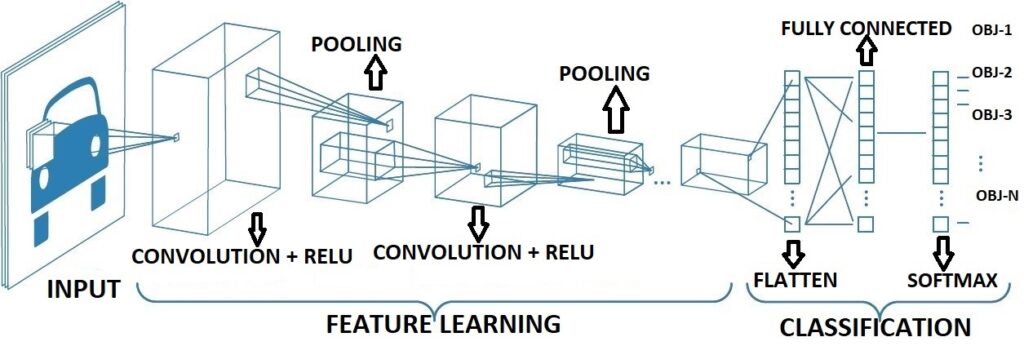
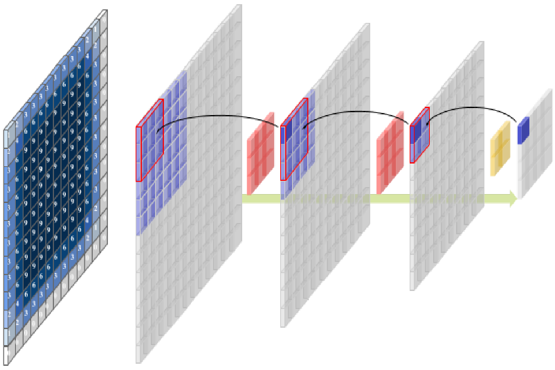
The fundamental presumption about the issues that CNN addresses is that they shouldn’t have spatially dependent aspects. To put it another way, don’t have to worry about where the faces are in the photographs in a facial recognition program. It doesn’t matter where they are in the surroundings; their discovery is the only thing that matters. Another crucial property of CNN is its ability to extract abstract properties when fed into advanced stages or deeper levels. For instance, in the first layer of picture classification, the edge may be detected, then simpler forms in the second layer, and finally higher-level characteristics [14]. Figure 1 provides an explanation of convolutional neural networks. A popular form of neural network is the CNN [15]. A CNN is similar to a multilayer perceptron (MLP) in concept. The activation function of every neuron in the MLP labeled with input and output weights. When add extra hidden layers after 1st layer to MLP, then it is called deep MLP. Similarly, CNN is regarded as an MLP with a unique structure. The architecture of the model permits CNN to be both translation and rotation invariant because of this particular structure [16]. In a CNN design, a convolutional layer, a pooling layer, and a comprehensively layer with a corrected activation function [17] are the three essential layers.

There are other methods for hyperspectral image classification that are competing in the literature. Some of these include:

1. Support vector machine (SVM)
2. Random forest (RF)
3. Principal Component Analysis (PCA)
4. Independent Component Analysis (ICA)
5. Deep Belief Networks (DBN)
6. Convolutional Auto encoder (CAE)
7. Generative Adversarial Networks (GANs)

The reason why Convolutional Neural Networks (CNNs), 2D and 3D CNNs, and hyperspectral imaging are encouraged in the literature is due to their ability to effectively capture the spectral and spatial information in hyperspectral images, leading to improved classification accuracy. In a variety of computer vision applications, such as picture classification, object recognition, and semantic segmentation, CNNs have demonstrated exceptional performance., among others. Additionally, 2D and 3D CNNs have been designed to take into account the spatial and spectral dimensions of hyperspectral images, leading to improved performance in hyperspectral image classification tasks. In comparison, traditional methods such as SVMs, RF, PCA, ICA, DBN, CAE, and GANs may not be as effective in capturing the complex relationships

between the spectral and spatial information in hyperspectral images, leading to lower classification accuracy. However, these methods still have their own advantages and are often used in combination with CNNs to address specific limitations and improve performance in hyperspectral image classification tasks.

CNN is a deep learning architecture that uses layers to classify things. It also included layers labelled as one input layer, numerous hidden layers, and one output layer. CNN works in the same way that DNN does, in that it takes input from a dataset, applies functions to it in the hidden layers, and then finds the result and displays it in the output layer. Max pooling, convolution, and fully linked layers are the most commonly employed CNN layers. The filter is convolved with input information in the layer of convolution.

The input is down sampled by the max pooling layer, and the input is fully connected by the fully connected layer, which connects all neurons from the previous layer to each other [18]. Now discuss the models of CNN that are in the form of 2D, 3D, and many more, but the focus will be on some major ones that are used for some classifications. By raising the number of layers, CNN is able to learn high-level hierarchical features. When the number of layers is increased, however, the input data or gradient starts to disappear. A more value-showing model, known as a dense convolutional network, was developed to overcome this problem (DenseNet). They devised a feed-forward algorithm that can interconnect each layer with every layer. Now expanded the feature set after being inspired by the thought that dense connections can boost feature utilization. For gesture recognition, 2-dimensional DenseNet to 3-dimensional DenseNet is used [19].

The spatial perspective, on the other hand, refers to the 2D spatial data about the objects that is present in hyperspectral images. As a result, hyperspectral pictures are frequently represented using 3D spectral-spatial data. As a result, the literature has provided a variety of approaches. Contrarily, current CNN-based algorithms [20] that only pay attention to spectral or spatial information are forced to ignore the connections between the spatial and spectral viewpoints of objects captured in hyperspectral pictures [21, 22].

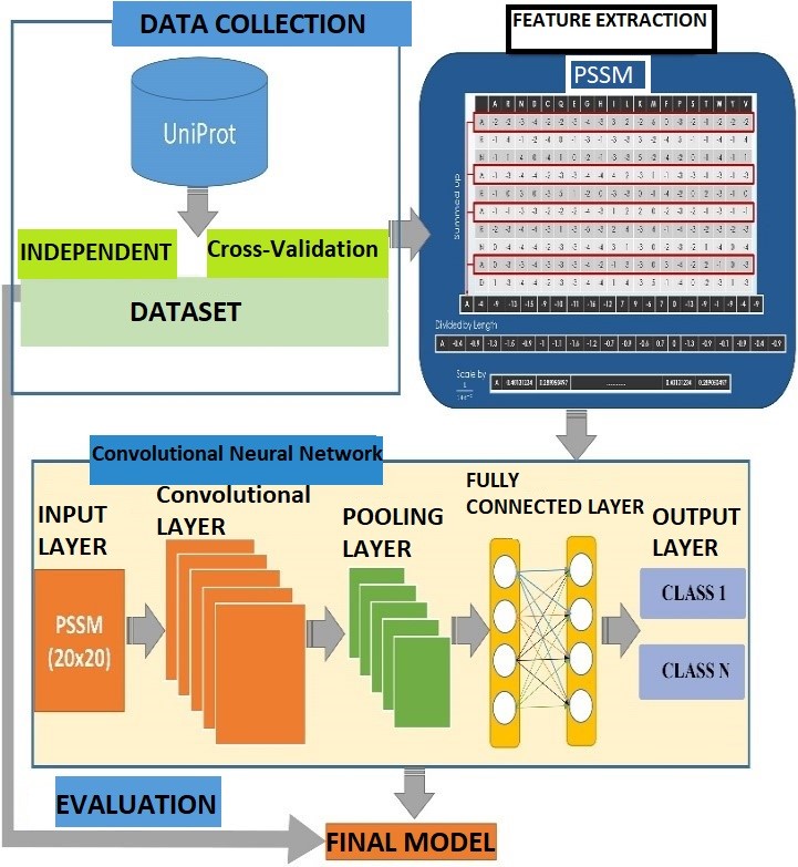
To extract features from these planes using three 2D CNNs, and then integrate three 2D network architectures in parallel, resulting in the multichannel 2D CNN. The 2D CNN model is made up of three elements of the 2D CNN architecture running in parallel, as well as a fully connected hidden unit that integrates multichannel data. Each 2D CNN takes only one sort of multichannel 2D image as an input and performs convolution computing on its own. The outputs from three 2D CNN sections are flattened, concatenated, and then fed into a fully connected neural network for learning. Finally, 2D CNN produces the categorization outcome. Given that the concatenation characteristics include features obtained from three orthogonal planes, 2D CNN considers 3D. As above figure 2 shows the architecture of 2D convolutional neural network for image classification by using proposed dataset with the function of feature extraction. Given that they may be used with either a series of 2D frames or a 3D volume as input, 3D CNNs are a complicated model for computational approaches for volumetric data (e.g. slices in a CT scan). Using 3D convolution kernels and 3D

pooling, methods that may be applied to volumetric data such as computed tomography (CT) images have been developed. The addition of 3D convolution kernels to the architecture increases the number of parameters, training time, and data requirements.

Training 3D CNNs on data from multiple methods is not always simple due to the limited size of medical picture datasets. Some pioneering attempts have been made along this line [23-28] to describe spectral and spatial information concurrently. 3D CNN models execute stacked convolution operations in a layer-by-layer way over spatial and spectral feature space. The generated rich feature maps are clearly the advantage of this type of 3D CNN model. These approaches, on the other hand, have three major drawbacks. To begin with, creating a more detailed 3D CNN model is tricky.

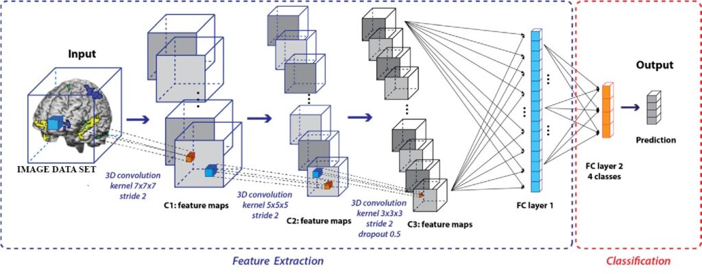
The reason for this is that as the number of 3D convolution processes rises, the solution space expands exponentially, limiting the model’s depth and interpretability. Second, if a significant number of 3D convolution operations are performed, the memory cost becomes prohibitive. Third, the small size of the public hyperspectral image datasets makes it impractical to train a deeper 3D CNN model, which requires extra training instances. To address the aforementioned issues, this work proposes a unique 3D CNN model that requires only a few 3D convolution operations but produces richer feature maps [29]. Figure 3 represents the 3D convolutional neural network architecture for image classification by using proposed dataset after extracting features from that proposed dataset.

1.2. Hyperspectral imaging

Hyperspectral images (HSIs), which contain hundreds of spectral bands, are created using a network of hyperspectral imaging sensors. Since there is a very tiny wavelength gap between every two nearby bands, HSIs have a very high spectral resolution [30]. (usually 10 nm). The use of HSI analysis is widespread in a variety of industries, including materials analysis, precision agriculture, environmental monitoring, and surveillance [31–33]. The hyperspectral community’s most active area of study is HSIs classification, which aims to categories every pixel in an image [34].

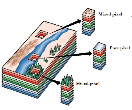
In figure 4 show the concept of hyperspectral imaging. The categorization of HSIs is challenging, nevertheless, due to the heavily duplicated spectral band information and few training samples [35]. In an HS image classification system, image restoration (e.g., de-noising, incomplete data restoration) [36,37], feature vectors [38], spectral un-mixing, and feature extraction [39] are all general sequential processes. Feature extraction is one of them, and it’s a vital stage in HS image categorization that’s been getting a lot of attention lately. A vast range of powerful hand-crafted and machine learning-based feature extraction techniques for HS image classification have been presented over the last decade [40]. These algorithms are capable of handling small-sample classification issues well. When the training size progressively expands and the training images become more complicated, they are likely to hit a performance bottleneck. This could be owing to the traditional approaches’ restricted data fitting and representation abilities.

2. Related Work review

In this article they used a three-dimensional convolutional neural network to classify lung nodules in chest CT images. In this proposed method they used two techniques one is screening stage and second is discrimination stage. A CAD system’s scanning stage is a standard feature. This stage narrows the initial search space and indicates a selection of the most likely candidates who should be investigated further. The screening CNN in our system is initially trained to classify 3D patches derived from each CT case using 3D convolution kernels [41]. The negative samples were chosen arbitrarily by extracting VOIs of the same size as the tested cases from a random location within the CT scan, whereas the specimens for this CNN were created by trying to extract VOIs of the same size as the tested cases from a random location inside the CT scan (in both the inside and outside of the lungs) (including both the  inside and outside of the lungs). The selection of the negative patches ensured that none of the  nodules would be overlapped by them. The number of negative samples obtained in this way may be nearly as big as required because the majority of the region within a chest CT is nodule-free. On the other hand, there are only a certain number of positive samples. The positive samples are reinforced by inserting flipped and rotated copies of each extracted positive patch in the training set to increase the system’s invariance to small variations in nodule appearance and to decrease the aforementioned class imbalance problem. The previous section’s screening stage still produces a significant percentage of false positives. The goal of the discriminating stage is to lower this number so that the clinician receives an output with high sensitivity for  nodule detection and a tolerable number of false positives per case. They trained their models using a subset of 509 cases from the LIDC dataset, with slice thicknesses ranging from 1.5 mm to 3 mm, as well as an extra 25 examples for testing. One to four radiologists indicate the location of each module in the LIDC dataset, and the radiologist provides a segmentation for each newly discovered 3 mm nodule.

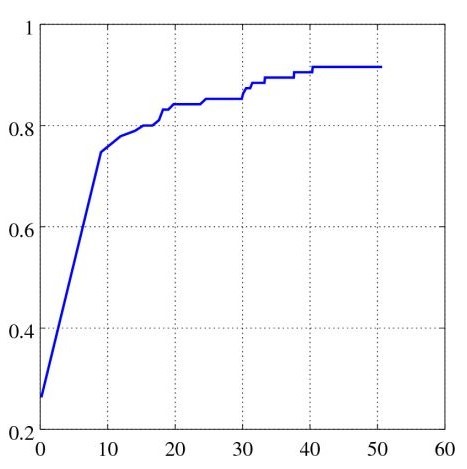
Only screening candidate points that pass the previously described criterion are used to evaluate the discriminatory CNN. The FROC curve for the discrimination stage is shown in Figure 4. At 15.28 FPs per case, this model achieves an 80% sensitivity. it suggests that this is accuracy is not much good as compare to other implementations of CNN, it can be improved by using other proposed methods for that we discussed is discussion session.

They suggested an approach for hyperspectral image categorization that employs an adaptive convolutional neural network. Their great performance is based on the spatial linkages being exploited by convolution kernels. As a result, filter design is critical for model performance. However, there are objects of various form and orientations in hyperspectral data, prohibiting filters from seeing “all imaginable” when making decisions [42]. The deeper neurons in the visual cortex are activated by several, more complicated inputs in a hierarchical manner, whereas the output neurons are triggered by some input visual stimulus that is within their RF. On the other hand, CNNs have changed their function to mirror this behaviour. The CNN employs a single deep stack of convolutional layers, each of which defines a filter bank, or a group of shareable, teachable, and locally connected weights that collectively form a linear n-dimensional kernel. A collection of data-fitted filters that sequentially traverse through the input data, overlap, and then apply themselves to the data make up the kernel.

The inputs that are included within the app’s region and the filter weights are combined to create a weight value for each application. Additionally, a non-linear activation function is added to reflect the convolution layer’s reaction to the search features in order to show if the features that were filtered by them are present (such as edges and forms).  Following equation defines this behaviour mathematically.

$$X_j^{(l)} = H\left( \sum_{k \in \mathbb{K}} X_{j+k}^{l-1} W_k^{(l)} \right) \tag{1}$$

Mathematical formula for a neural network operation in the forward propagation step. Where the superscript l indicates the Lth layer of a CNN, and in above equation H is usually implemented with ReLU and it denotes the activation function. Figure 2 illustrates this graphically. In particular, Figure 2b shows a 6 x 6 feature maps implemented with a 3 x 3 kernel with taking zero padding. In this case, k will test the input feature’s locations from (2, 4) to (4, 6) (some parts of padding provided to the border of map is included) that is based on K = [1, 1] according to grid for the end coordinate j = (3, 5, z). As can be seen, the output unit only depends on the kernel’s “seeing” of a small fraction of the input feature map. Any information contained in the input feature map that is outside of the RF has no bearing on the value of the output unit since this area has been designated as the RF for that unit [43].

By tracing the hierarchy back from the output feature under consideration to the input image, an effective receptive field (ERF) is established. The input data components that influence and modify the output activations are identified by the ERF. In this way, CNN’s ERF resembles a Gaussian distribution, designating an area to “look at” but also exponentially concentrating attention on the centre of the feature map. The soft attention map is really based on Gaussian distributions [44,45]. One of DL’s major achievements is the creation and use of the same neural architecture for the categorization of diverse pictures. The tests looked at the model’s complexity, accuracy, and generalizability by counting the number of parameters. identifying and categorizing the scenes from (i)the University of Pavia and (ii) the University of Houston, two authentic, well-known HSI sceneries with a variety of spectral-spatial properties. The information is given below.

• The University of Pavia dataset [46] is an HSI picture that was taken over the university’s campus in Pavia, northern Italy, in July 2002 using the ROSIS-3 airborne reflecting optics system imaging spectrometer. The picture consists of 113 wavelength channels with a frequency range of 430 to 860 nm and 610 × 340 pixels with a resolution of 1.3 m. The 42,776 tagged samples that make up the ground truth are separated into nine different land-cover classes, which include, among other urban features, asphalt, meadows, gravel, trees, steel plate, bare soil, bitumen, brickwork, and shadows.
• The lightweight tiny aerial spectrographic imager captured an HSI scene above the Houston University region for the University of Houston dataset [47] (CASI). It features 144 channels in the 380 nm to 1050 nm spectral range and 349 1905 pixels with a spatial resolution of 2.5 m. 15,029 tagged samples from 5 different courses in an urban setting are also part of the ground truth.

An innovative deep convolution-based neural network for the HSI classification process is presented in this study. The CNN classifier’s effective receptive field is automatically modified by the model’s deformable kernels and deformed convolutions to account for spatial deformations in HSI data from remote sensing. Instead of just being able to change the convolution, the adaptive classification network accomplishes this automatically by utilizing the distortion of the kernel itself applied to each perceptron on the input feature volume (i.e., adding an offset to the feature positions).

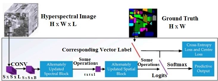
An upgraded spectral-spatial convolutional network has been offered as an alternate method for HSI classification. Figure 7 depicts the recommended method in broad strokes. A spatial size of S X S was selected from the raw HSI data in order to input HSI data with L channels and a size of H X W into the AUSSC network. The AUSSC picks up the spectral and spatial characteristics of an initial HSI patch using three separate convolutional kernels. The deep spectral and spatial features are modified by the alternately updated spectral and spatial blocks via recurrent feedback. The model parameters are enhanced by using the cross-entropy loss and center-loss loss functions [48]. The three 3D CNN algorithms—3D CNN, SSRN, and FDSSC—all show that a 3-dimensional edge framework outperforms 2D-CNN-based techniques and other deep learning-based approaches. This is due, among other things, to the fact that an end-to-end framework may reduce the amount of time it takes to complete a project. Reduce pre- and post-processing to ensure that the final output and original input have the closest possible relationships. Then, to increase the degree of fitness, the model is enlarged to include additional area that can be altered automatically by the data. additionally, when used with HSIs with a three-dimensional structure. In contrast to current CNN-based techniques, we offer an end-to-end CNN-based system that makes use of smaller convolutional kernels. The AUSSC employs kernels and disregards other architectures for categorizing HSI. The key distinction between the a m1 and a m2 convolutional kernels used in the 3D CNN technique is the spectral dimension. To learn spectral and spatial representations, SSRN uses spectral kernels of size 1 m and spatial kernels of size 1D, respectively. Convolutional kernels set the parameters for the model and govern which features the CNN learns. In InceptionV3, we introduce the idea of factorization into smaller convolutions [48].

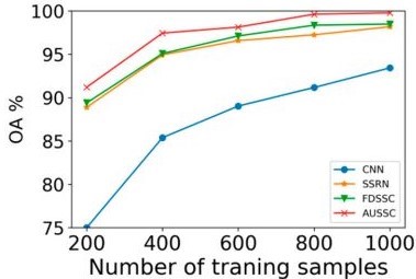
To illustrate that the suggested strategy may decrease data reliance, they employed a very small number of training samples (200). Insufficiently labelled data is unavoidable in remote sensing applications. Furthermore, remote sensing data collection and labelling is time-consuming and costly. Therefore, creating huge, high-quality label sets is really challenging. The number of labelled samples used for learning is the most crucial variable in deep-learning supervised techniques since data dependency is one of the most critical difficulties in deep learning.

In contrast to conventional machine-learning techniques, deep learning largely depends on extensive training data to recognized possible patterns. 200 training samples are required for semi-supervised 3D-GANs as well, although their classification performance is substantially lower. [49]. Revised spectral and spatial features in HSIs were used as the fundamental building blocks to develop an end-to-end CNN-based framework for HSI classification. To learn HIS qualities and combine them into advanced features, our concurrently updated convolutional spectral-spatial network uses spatial and spectral blocks that have been modified in the opposite direction. Our technique outperforms previous deep learning-based methods by learning deeply refined spectral and spatial characteristics via alternatively updated blocks, allowing it to attain high classification accuracy.

They said that the CNN is a multilayer neural network where the convolution layer, max – pooling, and fully – connected layers are all components. The CNN model’s convolution, which is the top layer, performs the convolution operation on the input data. Convolution involves performing an inner product operation on the kernel and receptive field of two matrices (learnable parameters). The feature map is constructed based on the input information and accessible features, and the kernel is often smaller than the original data and situated in the receptive field. The feature map’s dimension may be effectively decreased thanks to the pooling layer. The perceptron-like convolution layer, which is composed of neurons, is multilayered, has all of the neurons linked to one another, and the output characteristics are employed in the mapping. The features are mapped into the output using this layer. Researchers found that inter band correlation has a high level of redundancy in HSI analysis. Without suffering a considerable loss of information that may be used later, the data structure of the spectral dimension can be scaled down. Contrarily, an HSI consists of hundreds of spectral bands, which makes it more difficult for the network model to handle data while also using a large amount of processing power. In recent years, PCA has been widely employed in HSI classification studies to prepare the data.

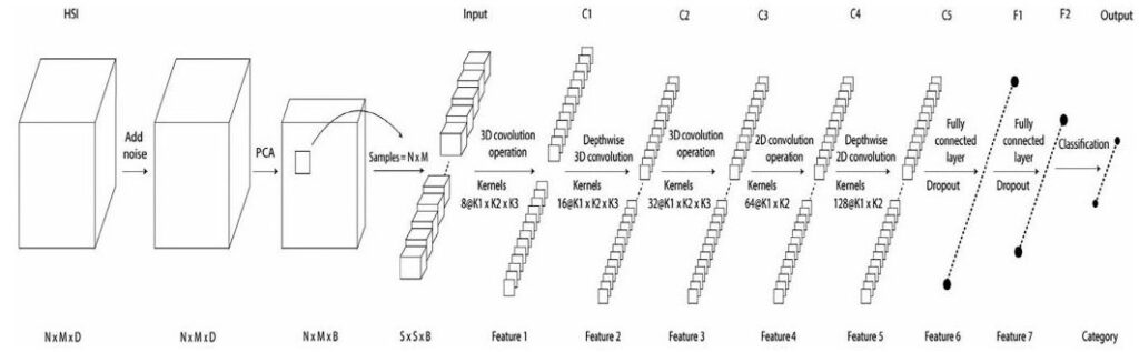
In accordance with HSI classifications, the two-dimensional complexity action takes into account the input data in the spatial dimension while the three-dimensional pre-processing phase analyses the input data concurrently in the spatial and spectral dimensions. For HSIs with rich spectral information, the capacity to maintain the spectrum information of the incoming HSI data via 3-D convolution is crucial. However, whether two-dimensional convolution procedures are performed on two-dimensional or three-dimensional data, the end output is always two-dimensional, regardless of whether two-dimensional convolution techniques are employed on the HSI or not.  The suggested method effectively recovers high-quality spectral and spatial feature maps from the HSI by merging the 3-D CNN and 2-D CNN. A diminishing dimension block (a Conv3-D + reshaping operation + a Conv3-D), a 3-D stacked convolution layer (a Conv3-D – fast learning layer), and ultimately a 3-D stacked convolution layer (a Conv3-D) are all used in the proposed model

From which the output feature maps are then reshaped and supplied to a Conv2-D to learn more spatial information. The output of the Conv2-layer is flattened before it is sent to the top fully connected layer.  A dropout layer comes after the last fully linked layer. The proposed model’s 3-D fast learning CNN block is significantly less computationally expensive and faster than the ordinary block due to the inclusion of depth-wise separable convolution and the fast convolution block in the fast learning block. To employ image classification algorithms, hyperspectral data cubes for input are split into tiny 3-D patches called PRSB, whose center pixel determines the class labels. Initially, the size of the right N m labels matched the quantity of input data patches. Although the correct labels contain a background, we transmit the data to the network as input after removing the background from the labels and patches. The convolution layer in the input image is composed of a sliding kernel. To extract important feature maps from the input, this kernel has weights that change throughout training. These qualities are used in the categorization process. The number of HSIs available is insufficient, and data is scarce. Designing a model that matches the environment is one of the hurdles in categorizing HSIs. This research provides a hybrid model of 3-D and 2-D convolution for HSI classification. To improve classification performance, spatial and spectral characteristics might be employed. In the hybrid model, the spatial-spectral information and spatial information obtained via 3-D and 2-D convolution, respectively, are integrated.

Figure 9 depicts the suggested method’s design. As opposed to employing 3-D-CNN alone, combining 3-D-CNN with 2-D-CNN reduces the number of learning parameters while also using less processing power. The Adam optimizer does a better job at network optimization and cuts down on training time. In comparison to other models, the hybrid model has the best performance in terms of limiting the number of training samples and noise. We may increase the number of layers in the model and deepen the network after we have a sufficient amount of training data. Although all models have good accuracy Due to the hybrid structure’s capability to exploit all of the spectral and spatial information in HSI data, the hybrid model has fewer parameters and takes less training time than the 3-D-CNN model and the 2-D-CNN model when sufficient training instances are available. Because of this, utilizing a hybrid model for HSI categorization is economical. [50] proposed a system that is implemented Artificial Neural Network for classification of FPGA cart Flower.  The recommended method’s superiority in the face of a short training sample and noise was confirmed by experiments on three datasets using three classification algorithms that  were compared.

3. Material and Methods

The material and methods that are discussed and used in the assessed articles are based on 2D and 3D hyperspectral images and methods are mainly based on CNN. The data is collected from various sources, such as airborne or satellite sensors, and pre-processing the data to remove noise, correct atmospheric effects, and extract relevant features. Then extract relevant features from the hyperspectral data to represent the spectral-spatial information, such as using principal component analysis (PCA), independent component analysis (ICA), or texture features. The select and implement the model, in this article the main focus is on the implementation of convolutional neural network model that is mostly used for the image classification. Then train the selected deep learning model using annotated hyperspectral data, some of papers are in a supervised and some are unsupervised manner. After training evaluate the performance of the trained model using metrics such as accuracy, F1-score, precision, recall, and confusion matrix. Then implement the fine-tuning the parameters of the trained model to improve its performance, such as adjusting the regularization strength, changing the kernel function, or adding more hidden layers. The materials required for hyperspectral image classification include a computer with sufficient computational power, deep learning libraries such as Tensor-Flow or Py-Torch, and annotated hyperspectral data. Additionally, a software tool such as MATLAB or Python can be used to implement the algorithms and evaluate the performance of the models.

A systematic approach to using Convolutional Neural Networks (CNNs) would include the following steps:

• Define the problem: Determine the task you want to solve and the type of data you have available.
• Preprocess the data: Clean, normalize, and prepare the data for use in the CNN. This may include converting images to grayscale, resizing, and splitting the data into training, validation, and testing sets.
• Choose a CNN architecture: Select an appropriate CNN architecture based on the type of data you have and the task you want to solve. Common CNN architectures include Le-Net, Alex-Net, VGG-Net, Res-Net, and Inception-Net.
• Train the model: Train the model on the training data, using an optimization algorithm such as stochastic gradient descent (SGD) or Adam, and a loss function such as mean squared error (MSE) or cross-entropy.
• Validate the model: Evaluate the performance of the model on the validation data. This is used to tune the hyper-parameters of the model, such as the learning rate and batch size.
• Test the model: Evaluate the performance of the model on the test data. This provides an estimate of how well the model will perform on unseen data.
• Deploy the model: Deploy the trained model in a production environment, using a framework such as Tensor-Flow or Py-Torch.
• Monitor performance: Regularly monitor the performance of the deployed model and make improvements as necessary.

4. Results and Discussion

In this paper, we have reviewed and critically compared many supervised hyperspectral classification approaches from multiple perspectives, with a focus on the setup, speed, and automation capabilities of various algorithms. Popular approaches such as SVMs, neural networks (2D and 3D convolutional neural network), and deep approaches are among the techniques compared, which have been widely employed in the hyperspectral analysis field but have never been comprehensively investigated using a quantitative and comparative methodology. The article lies in its focus on the recent advancements in the classification of hyperspectral images using 2D and 3D convolutional neural networks (CNNs)  with channel and spatial attention mechanisms. The review summarizes the current state-of-the-art methods and provides insights into the latest developments in the field, highlighting the strengths and limitations of different approaches. The key conclusion that can be drawn from this research is that no classifier consistently gives the greatest performance among the criteria under consideration (particularly from the viewpoint of classification accuracy). Different solutions, on the other hand, are dependent on the complexity of the analysis scenario (for example, the availability of training samples, processing needs, tuning parameters, and algorithm speed) as well as the application domain in question. The informative analysis of all the reviewed papers given in below table.

Table 1: Comparison of different methods for Hyperspectral Image classification

5. Conclusion

To advance the field of classification of hyperspectral images using 2D and 3D CNNs with channel and spatial attention, the following open research challenges and future research directions can be considered:

Finding more effective ways to exploit the rich spectral-spatial information in hyperspectral images to improve classification accuracy. Generalization to real-world scenarios: Improving the generalization of CNN models to real-world hyperspectral data, which can often be noisy and have complex background variations. Combining multiple sources of information:

Exploring the integration of other sources of information, such as elevation data or textual annotations, to improve hyperspectral image classification performance. Computational efficiency:

Developing more efficient algorithms to reduce the computational burden of hyperspectral image classification, especially for large-scale datasets. Robustness to atmospheric and illumination conditions:

Improving the robustness of CNN models to variations in atmospheric conditions and illumination, which can significantly impact the performance of hyperspectral image classification.

Semi-supervised and unsupervised learning: Investigating the potential of semi-supervised and unsupervised learning methods for hyperspectral image classification to reduce the need for large annotated datasets. Exploring the use of multi-scale information to improve the classification of hyperspectral images, such as using multi-scale convolutional filters or combining multiple CNNs with different receptive field size. This work will be enhanced by the use of other suitable methodologies for the categorization of hyperspectral pictures, such as Transformers, which will be dependent on his/her expectations and/or exploitation aims.

Conflict of Interest

The authors declare no conflict of interest.

1. Yin, J.; Qi, C.; Chen, Q.; Qu, J. Spatial-Spectral Network for Hyperspectral Image Classification: A 3- D CNN and Bi-LSTM Framework. Remote Sens. 2021, 13, 2353, org/10.3390/rs13122353.
2. Yan, H.; Wang, J.; Tang, L.; Zhang, E.; Yan, K.; Yu, ; Peng, J. A 3D Cascaded Spectral–Spatial Element Attention Network for Hyperspectral Image Classification. Remote Sens. 2021, 13, 2451, doi.org/10.3390/rs13132451.
3. Pu, S.; Wu, Y.; Sun, X.; Sun, X. Hyperspectral Image Classification with Localized Graph Convolutional Filtering. Remote Sens. 2021, 13, 526, org/10.3390/rs13030526.
4. Hong, D.; Yokoya, N.; Chanussot, J.; Zhu, X.X. An Augmented Linear Mixing Model to Address Spectral Variability for Hyperspectral Unmixing. IEEE Trans. Image Process. 2019, 28, 1923–1938, DOI: 1109/TIP.2018.2878958.
5. Gudmundsson, Steinn, Thomas Philip Runarsson, and Sven Sigurdsson. “Support vector machines and dynamic time warping for time series.” 2008 IEEE International Joint Conference on Neural Networks (IEEE World Congress on Computational Intelligence). IEEE, 2008.Wang, Q.; Meng, Z.; Li, X. Locality adaptive discriminant analysis for spectral–spatial classification of hyperspectral images. IEEE Geosci.                   Remote Sens. Lett. 2017, 14, 2077–2081, DOI: 1109/IJCNN.2008.4634188.
6. Wang, Q.; Lin, J.; Yuan, Y. Salient band selection for hyperspectral image classification via manifold ranking. IEEE Trans. Neural Netw. Learn. Syst. 2016, 27, 1279–1289, DOI: 1109/TNNLS.2015.2477537.
7. He, K.; Zhang, X.; Ren, S.; Sun, J. Deep residual learning for image recognition. In Proceedings of the IEEE Conference on Computer Vision and Pattern Recognition, Las Vegas, NV, USA, 27–30 June 2016; pp.770–778, DOI: 1109/CVPR.2016.90.
8. Sharma, V.; Diba, A.; Tuytelaars, T.; Van Gool, L. Hyperspectral CNN for Image Classification & Band           Selection, with Application to Face Recognition; KU                  Leuven, ESAT: Leuven, Belgium, 2016, org/10.3390/pr11020435.
9. Krizhevsky, A.; Sutskever, I.; Hinton, G.E. Imagenet classification with deep convolutional neural networks. In Advances in Neural Information Processing Systems; Curran Associates, Inc.: New York, NY, USA, 2012; pp. 1097–1105, org/10.1145/3065386.
10. Goodfellow, Ian, Yoshua Bengio, and Aaron  Deep learning. MIT press, 2016.
11. Albawi, Saad, Tareq Abed Mohammed, and Saad Al-Zawi. “Understanding of a convolutional neural network.” 2017 International Conference on Engineering and Technology (ICET). Ieee, 2017, DOI:1109/ICENGTECHNOL.2017.8308186.
12. Schmidhuber, “Deep Learning in neural networks: An overview,” Neural Networks, vol. 61. pp. 85–117, 2015, doi.org/10.1016/j.neunet.2014.09.003.
13. Zhao, H. Lu, S. Chen, J. Liu, and D. Wu, “Convolutional neural networks for time series classification,” J. Syst. Eng. Electron., vol. 28, no. 1,    pp. 162–169, 2017, DOI: 10.21629/JSEE.2017.01.18.
14. He, X. Zhang, S. Ren, and J. Sun, “Delving deep into rectifiers: Surpassing human-level performance           on imagenet classification,” in Proceedings of the   IEEE International Conference on Computer Vision,           2016, vol. 11–18–Dece, pp. 1026–1034, doi.org/10.48550/arXiv.1502.01852.
15. Aslam, M. A., Sarwar, M. U., Hanif, M. K., Talib, R., & Khalid, U. (2018). Acoustic classification using deep learning. Int. J. Adv. Comput. Sci. Appl, 9(8), 153-159,  (DOI) : 14569/IJACSA.2018.090820.
16. Huang, G.; Liu, Z.; Van Der Maaten, L.; Weinberger, K.Q. Densely connected convolutional networks. In Proceedings of the 30th IEEE Conference on Computer Vision and Pattern Recognition (CVPR   2017), Honolulu, HI, USA, 21–26 July 2017; pp.           2261–2269, DOI: 1109/CVPR.2017.243.
17. Hu, J., Kuang, Y., Liao, B., Cao, L., Dong, S., & Li, (2019). A multichannel 2D convolutional neural network model for task-evoked fMRI data classification. Computational intelligence and neuroscience, 2019, doi.org/10.1155/2019/5065214.
18. Liu, B.; Yu, X.; Zhang, P.; Tan, X.; Yu, A.; Xue, Z. A semi-supervised convolutional neural network for
    hyperspectral image classification. Remote Sens. Lett. 2017, 8, 839–848, org/10.1080/2150704X.2017.1331053.
19. Yang, X.; Ye, Y.; Li, X.; Lau, R.Y.; Zhang, X.; Huang, Hyperspectral Image Classification with Deep
    Learning Models. IEEE Trans. Geosci. Remote Sens. 2018, 56, 5408–5423, DOI: 10.1109/TGRS.2018.2815613.
20. Hamida, A.B.; Benoit, A.; Lambert, P.; Amar, C.B. 3- D Deep Learning Approach for Remote Sensing          Image Classification. IEEE Trans. Geosci. Remote Sens. 2018, 56, 4420–4434, DOI: 1109/TGRS.2018.2818945.
21. Li, Y.; Zhang, H.; Shen, Q. Spectral–spatial classification of hyperspectral imagery with 3D convolutional neural network. Remote Sens. 2017, 9, 67, org/10.3390/rs9010067.
22. He, M.; Li, B.; Chen, H. Multi-scale 3D deep convolutional neural network for hyperspectral image
    In Proceedings of the 2017 IEEE International Conference on Image Processing (ICIP), Beijing, China, 17–20 September 2017; pp.3904–3908, DOI: 10.1109/ICIP.2017.8297014.
23. Luo, Y.; Zou, J.; Yao, C.; Zhao, X.; Li, T.; Bai, G. HSI-CNN: A Novel Convolution Neural Network for
    Hyperspectral Image. In Proceedings of the 2018 International Conference on Audio, Language and           Image Processing, Shanghai, China, 16–17 July 2018;                 464–469, DOI: 10.1109/ICALIP.2018.8455251.
24. Fan, J.; Tan, H.L.; Toomik, M.; Lu, S. Spectral–spatial hyperspectral image classification using
    super-pixel-based spatial pyramid representation. In Proceedings of the Image and Signal Processing
    for Remote Sensing XXII, Edinburgh, UK, 26–29 September 2016; Volume 10004, pp.315–321, org/10.3390/rs12122033.
25. Yang, X., Zhang, X., Ye, Y., Lau, R. Y., Lu, S., Li, , & Huang, X. (2020). Synergistic 2D/3D           convolutional neural network for hyperspectral image classification. Remote Sensing, 12(12), 2033, doi.org/10.3390/rs12122033.
26. Wang, Q.; He, X.; Li, X. Locality and structure regularized low rank representation for hyperspectral image classification. IEEE Trans. Geosci. Remote Sens. 2018, 57, 911–923, DOI: 1109/TGRS.2018.2862899.
27. Yuan, Y.; Feng, Y.; Lu, X. Projection-Based NMF for Hyperspectral Unmixing. IEEE J. Sel. Top. Appl. Earth Obs. Remote Sens. 2015, 8, 2632–2643, DOI: 1109/JSTARS.2015.2427656.
28. Li, W.; Du, Q.; Zhang, B. Combined sparse and collaborative representation for hyperspectral target Pattern Recognit. 2015, 48, 3904–3916, doi.org/10.1016/j.patcog.2015.05.024.
29. Pan, B.; Shi, Z.; Xu, X. MugNet: Deep learning for hyperspectral image classification using limited samples. ISPRS J. Photogramm. Remote Sens. 2018, 145, 108–119, org/10.1016/j.isprsjprs.2017.11.003.
30. Zhou, S.; Xue, Z.; Du, P. Semisupervised Stacked Autoencoder with Cotraining for Hyperspectral Image Classification. IEEE Trans. Geosci. Remote Sens. 2019, 57, 3813–3826, DOI: 1109/TGRS.2018.2888485.
31. Ghamisi, P.; Plaza, J.; Chen, Y.; Li, J.; Plaza, A.J. Advanced Spectral Classifiers for Hyperspectral Images: A review. IEEE Geosci. Remote Sens. Mag. 2017, 5, 8–32, DOI: 1109/MGRS.2016.2616418.
32. Cao, K. Wang, G. Han, J. Yao, and A. Cichocki, “A robust pca approach with noise structure learning           and spatial–spectral low-rank modeling for               hyperspectral image restoration,” IEEE J. Sel. Top. Appl. Earth Obs. Remote Sens., vol. 11, no. 10, pp.3863–3879, 2018, DOI: 10.1109/JSTARS.2018.2866815.
33. Hong, N. Yokoya, J. Chanussot, J. Xu, and X. X. Zhu, “Joint and progressive subspace analysis (jpsa)           with spatial-spectral manifold alignment for semi-supervised hyperspectral dimensionality reduction,”
    IEEE Trans. Cybern., vol. 51, no. 7, pp. 3602–3615,            2021, DOI: 10.1109/TCYB.2020.3028931.
34. Luo, T. Guo, Z. Lin, J. Ren, and X. Zhou, “Semisupervised hypergraph discriminant learning for dimensionality reduction of hyperspectral image,” IEEE J. Sel. Top. Appl. Earth Obs. Remote Sens., vol. 13, pp. 4242–4256, 2020, DOI: 10.1109/JSTARS.2020.3011431.
35. Hong, X. Wu, P. Ghamisi, J. Chanussot, N. Yokoya, and X. X. Zhu, “Invariant attribute profiles: A spatial-frequency joint feature extractor for hyperspectral image classification,” IEEE Trans. Geosci. Remote Sens., vol. 58, no. 6, pp. 3791–3808,              2020, doi: 10.1109/TGRS.2019.2957251.
36. Rasti, D. Hong, R. Hang, P. Ghamisi, X. Kang, J. Chanussot, and J. Benediktsson, “Feature extraction for hyperspectral imagery: The evolution from shallow to deep: Overview and toolbox,” IEEE Geosci. Remote Sens. Mag., vol. 8, no. 4, pp. 60–88, 2020, DOI: 10.1109/MGRS.2020.2979764.
37. Hamidian, S., Sahiner, B., Petrick, N., & Pezeshk, A. (2017, March). 3D convolutional neural network for automatic detection of lung nodules in chest CT. In Medical Imaging 2017: Computer-Aided Diagnosis (Vol. 10134, p. 1013409). International Society for Optics and Photonics, DOI: 1117/12.2255795.
38. Paoletti, M. E., & Haut, J. M. (2021). Adaptable Convolutional Network for Hyperspectral Image Classification. Remote Sensing, 13(18), 3637, Dorg/10.3390/rs13183637.
39. Le, H.; Borji, A. What are the receptive, effective receptive, and projective fields of neurons in convolutional neural networks? arXiv 2017, arXiv:1705.07049, org/10.48550/arXiv.1705.07049.
40. Gao, H.; Zhu, X.; Lin, S.; Dai, J. Deformable Kernels: Adapting Effective Receptive Fields for Object Deformation. arXiv 2019 ,arXiv:1910.02940, org/10.48550/arXiv.1910.02940.
41. Araujo, A.; Norris, W.; Sim, J. Computing receptive fields of convolutional neural networks. Distill 2019,           4, e21, DOI: 23915/distill.00021.
42. Xu, X., Li, J., & Plaza, A. (2016, July). Fusion of hyperspectral and LiDAR data using morphological component analysis. In 2016 IEEE International Geoscience and Remote Sensing Symposium (IGARSS), (pp.3575-3578). DOI: 1109/IGARSS.2016.7729926.
43. Wang, W., Dou, S., & Wang, S. (2019). Alternately updated spectral–spatial convolution network for the classification of hyperspectral images. Remote Sensing, 11(15), 1794, org/10.3390/rs11151794.
44. Szegedy, C., Vanhoucke, V., Ioffe, S., Shlens, J., & Wojna, Z. (2016). Rethinking the inception architecture for computer vision. In Proceedings of the       IEEE conference on computer vision and pattern    recognition (pp. 2818-2826), org/10.48550/arXiv.1512.00567.
45. Zhu, L., Chen, Y., Ghamisi, P., & Benediktsson, J. A. (2018). Generative adversarial networks for hyperspectral image classification. IEEE Transactions on Geoscience and Remote Sensing, 56(9), 5046- 5063, doi:1109/TGRS.2018.2805286.
46. Ghaderizadeh, S., Abbasi-Moghadam, D., Sharifi, A., Zhao, N., & Tariq, A. (2021). Hyperspectral image classification using a hybrid 3D-2D convolutional neural networks. IEEE Journal of Selected Topics in Applied Earth Observations and Remote Sensing, 14, 7570-7588, DOI:1109/JSTARS.2021.3099118.
47. Paoletti, J. Haut, J. Plaza, and A. Plaza, “Deep&dense convolutional neural network for hyperspectral image classification,” Remote Sens., vol. 10, 2018, Art. no. 1454, doi.org/10.3390/rs10091454.
48. Gao, S. Lim, and X. Jia, “Hyperspectral image classification using convolutional neural networks and multiple feature learning,” Remote
    Sens., vol. 10, no. 2, 2018, Art. no. 299, doi:10.3390/rs10020299.
49. Farooq, Umar, and Robert B. Bass. “Frequency Event Detection and Mitigation in Power Systems: A Systematic Literature Review.” IEEE Access 10 (2022), DOI: 10.1109/ACCESS.2022.3180349.
50. Ahmad, M. F., et al. “Tracking system using artificial neural network for FPGA cart follower.” Journal of Physics: Conference Series. Vol. 1874. No. 1. IOP Publishing, 2021, DOI 10.1088/1742-6596/1874/1/01.

Citations by Dimensions

Citations by PlumX

Crossref Citations

1. Muhammad Ahsan Aslam, Muhammad Tariq Ali, Sunwan Nawaz, Saima Shahzadi, Muhammad Ali Fazal, “Binary Image Classification with CNNs, Transfer Learning and Classical Models “, Journal of Engineering Research and Sciences, vol. 5, no. 1, pp. 66–75, 2026. doi: 10.55708/js0501006
2. Muhammad Ahsan Aslam, Muhammad Tariq Ali, Sunwan Nawaz, Saima Shahzadi, Muhammad Ali Fazal, “Model Uncertainty Quantification: A Post Hoc Calibration Approach for Heart Disease Prediction “, Journal of Engineering Research and Sciences, vol. 4, no. 12, pp. 25–54, 2025. doi: 10.55708/js0412003
3. Muhammad Ahsan Aslam, Muhammad Tariq Ali, Sunwan Nawaz, Saima Shahzadi, Muhammad Ali Fazal, “Comparative Analysis of Supervised Machine Learning Models for PCOS Prediction Using Clinical Data”, Journal of Engineering Research and Sciences, vol. 4, no. 6, pp. 16–26, 2025. doi: 10.55708/js0406003
4. Muhammad Ahsan Aslam, Muhammad Tariq Ali, Sunwan Nawaz, Saima Shahzadi, Muhammad Ali Fazal, “Fire Type Classification in the USA Using Supervised Machine Learning Techniques”, Journal of Engineering Research and Sciences, vol. 4, no. 6, pp. 1–8, 2025. doi: 10.55708/js0406001
5. Muhammad Ahsan Aslam, Muhammad Tariq Ali, Sunwan Nawaz, Saima Shahzadi, Muhammad Ali Fazal, “AI-Driven Digital Transformation: Challenges and Opportunities”, Journal of Engineering Research and Sciences, vol. 4, no. 4, pp. 8–19, 2025. doi: 10.55708/js0404002