Binary Image Classification with CNNs, Transfer Learning and Classical Models
(This article belongs to the Special Issue on Special Issue on Multidisciplinary Sciences and Advanced Technology 2025 and the Section Artificial Intelligence – Computer Science (AIC))
Export Citations
Cite
Oikonomou, N. V. , Oikonomou, D. V. , Chaliasou, S. P. and Rigas, N. (2026). Binary Image Classification with CNNs, Transfer Learning and Classical Models. Journal of Engineering Research and Sciences, 5(1), 66–75. https://doi.org/10.55708/js0501006
Nikolaos Vasileios Oikonomou, Dimitrios Vasileios Oikonomou, Sofia Panagiota Chaliasou and Nikolaos Rigas. "Binary Image Classification with CNNs, Transfer Learning and Classical Models." Journal of Engineering Research and Sciences 5, no. 1 (January 2026): 66–75. https://doi.org/10.55708/js0501006
N.V. Oikonomou, D.V. Oikonomou, S.P. Chaliasou and N. Rigas, "Binary Image Classification with CNNs, Transfer Learning and Classical Models," Journal of Engineering Research and Sciences, vol. 5, no. 1, pp. 66–75, Jan. 2026, doi: 10.55708/js0501006.
1.Introduction
Automated image classification has evolved into a central problem in computer vision, driven by the need to efficiently process vast amounts of visual data in applications ranging from biometric security to emotion recognition. While early approaches relied on handcrafted features, the advent of Convolutional Neural Networks (CNNs) revolutionized the field by enabling models to learn hierarchical feature representations directly from raw pixel data. Seminal architectures such as AlexNet and ResNet demonstrated that deep networks, utilizing techniques like ReLU activations and Dropout, could achieve breakthrough accuracy on massive datasets like ImageNet [1], [2].
However, deploying deep learning models for specific tasks, such as binary face classification, presents significant challenges. Training deep architectures from scratch requires substantial computational resources, large, labeled datasets, and meticulous hyperparameter tuning to avoid overfitting. Conversely, Transfer Learning strategies, which leverage pre-trained networks (e.g., ResNet50) as feature extractors, offer a compelling alternative by transferring knowledge from generic domains to specific tasks [3]. When combined with classical machine learning classifiers like Random Forests (RF) or Logistic Regression (LR), these approaches can potentially offer a balance between high accuracy and low training cost [4].
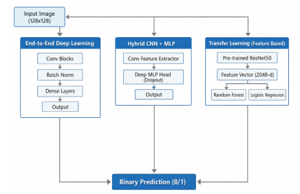
The primary motivation of this study is to navigate the trade-offs between computationally intensive End-to-End Deep Learning and efficient Feature-Based Classical Learning in the context of binary face classification. Specifically, we address the challenge of classifying face images into two categories using a dataset derived from a Kaggle challenge. A key issue investigated is the phenomenon of model generalization versus overfitting: while complex CNNs often struggle with underfitting when heavily regularized, feature-based classical models may exhibit near-perfect training accuracy but varying degrees of validation performance. The overall architectural pipeline designed for this comparative study, encompassing the end-to-end, hybrid, and transfer learning workflows, is visually summarized in Figure 1.
Unlike previous studies that typically focus on a single modeling paradigm, this work provides a rigorous comparative analysis across three distinct methodologies: (1) End-to-End CNNs (comparing a baseline TensorFlow implementation against an optimized PyTorch pipeline), (2) Hybrid CNN-MLP architectures, and (3) Transfer Learning coupled with classical classifiers.
The specific contributions of this paper are as follows:
- Framework and Optimization Analysis: We explicitly compare a standard TensorFlow/Keras baseline against a custom PyTorch-based CNN (“MyDeepCNN”). We demonstrate that the superior performance of the latter is driven not merely by the framework, but by an optimized training pipeline incorporating AdamW optimizer, Cosine Annealing learning-rate scheduling, and LeakyReLU activations.
- Evaluation of Feature-Based Classifiers: We show that combining deep features from a pre-trained ResNet50 with traditional classifiers (Random Forest, Logistic Regression) yields competitive or superior validation accuracy (>90%) and AUC (>0.97) compared to end-to-end CNNs, with a fraction of the training time.
- Critical Analysis of Overfitting/Underfitting: We provide a detailed examination of the training dynamics, explaining the “underfitting paradox” observed in the baseline CNN (where training accuracy lags behind in validation accuracy due to heavy augmentation) versus the massive capacity of Random Forests to fit training data perfectly.
The remainder of this paper is organized as follows: Section 2 reviews the theoretical background of CNNs, transfer learning, and regularization techniques. Section 3 details the dataset, preprocessing steps, and the specific architectures implemented (Baseline CNN, Hybrid Models, and Feature Extraction pipelines). Section 4 presents the experimental results, including metrics such as Accuracy, F1-score, and AUC-ROC, alongside confusion matrices. Section 5 discusses the findings, analyzing the trade-offs between deep and classical methods. Finally, Section 6 concludes the study and suggests directions for future research.
2. Theoretical Background
2.1. Convolutional Neural Networks (CNNs)
Convolutional Neural Networks (CNNs) have established themselves as the dominant architecture for visual recognition tasks due to their ability to capture spatial hierarchies in images through learnable filters [1]. A typical CNN architecture comprises alternating convolutional layers, which extract local features (e.g., edges, textures), and pooling layers that reduce spatial dimensionality and computational load.
To facilitate the training of deep architectures, modern CNNs incorporate Batch Normalization (BN). BN normalizes the inputs of each layer layer-wise, mitigating the problem of internal covariate shift. This allows for higher learning rates and acts as a regularizer, significantly accelerating convergence [5]. Furthermore, activation functions such as the Rectified Linear Unit (ReLU) and its variants (e.g., LeakyReLU) are standard in overcoming the vanishing gradient problem in deep networks [1].
2.2. Transfer Learning and Pre-trained Models
Training deep CNNs from scratch requires massive datasets to avoid overfitting. Transfer Learning addresses this by leveraging models pre-trained on large-scale datasets (e.g., ImageNet) to solve related tasks. Research indicates that the initial layers of CNNs learn generic features applicable across diverse domains, while deeper layers capture task-specific semantics [3].
In this study, we utilize ResNet50 [2], a 50-layer residual network, as a feature extractor. We also reference modern efficient architectures like EfficientNet, which optimize accuracy and efficiency through compound scaling [6], as benchmarks for future improvements. By extracting feature vectors from the penultimate layer of these models, we transform raw images into high-level semantic embeddings suitable for classical classification.
2.3. Classical Machine Learning Classifiers
While Deep Learning excels in end-to-end feature learning, classical classifiers offer advantages in interpretability and training speed when provided with high-quality features.
- Random Forest (RF): An ensemble learning method that constructs a multitude of decision trees at training time. It is robust to noise and overfitting (compared to individual decision trees) and provides insights into feature importance [4].
- Logistic Regression (LR): A linear model that estimates the probability of a binary outcome using the sigmoid function. Despite its simplicity, LR can achieve state-of-the-art performance when the input feature space (e.g., from ResNet50) is linearly separable.
2.4. Regularization and Optimization
To ensure robust generalization, especially in binary face classification where datasets may be limited, rigorous regularization strategies are essential.
- Data Augmentation: We employ geometric transformations (rotation, flipping, zooming) to artificially expand the training set and enforce invariance to input variations. Recent surveys highlight augmentation as a critical component for successful deep learning training [7].
- Optimization Algorithms: We utilize the Adam optimizer (Adaptive Moment Estimation), which computes adaptive learning rates for each parameter. For our optimized PyTorch model, we specifically use AdamW, a variant that decouples weight decay from gradient updates, offering superior regularization for deep models [8].
3. Methodology
3.1. Dataset Description and Preprocessing
The experimental evaluation utilized a dataset derived from the “Kaggle Face Classification Challenge”, specifically curated for binary classification tasks (Class 0 versus Class 1) [9].
- Data Volume and Splitting: The complete dataset comprises 6,376 facial images. To ensure robust model evaluation and prevent data leakage, we employed a stratified splitting strategy. The data was partitioned into a Training Set of 5,102 images (approx. 80%) and a Validation Set of 1,274 images (approx. 20%). Stratification was strictly applied to maintain the same class distribution in both subsets as in the original dataset, preventing bias during the training phase [10].
- Image Properties: The original images varied in resolution and lighting conditions. To standardize the input for the neural networks, all images were resized to fixed spatial dimensions of 128 Χ128 pixels with 3 color channels (RGB).
- Normalization: Prior to ingestion by the models, pixel intensity values were scaled from the integer range [0, 255] to the floating-point range [0, 1] by dividing by 255.0. This normalization step is critical for ensuring numerical stability and accelerating gradient descent convergence by keeping the input values within a small, bounded range [11].
3.2. Data Augmentation Strategy
Given the restricted size of the training dataset (N ≈5,100), the risk of the model memorizing specific training examples (overfitting) rather than learning generalizable features was significant. To address this, we implemented a robust Online Data Augmentation pipeline. Unlike offline augmentation, which expands the dataset size statically, online augmentation applies stochastic transformations to each batch of images dynamically during training. This ensures that the network never encounters the exact same image tensor twice, effectively simulating a vastly larger dataset [12].
The augmentation policy was carefully designed to simulate realistic variations in facial pose and lighting conditions without altering the semantic label of the image. The specific transformations applied are categorized as follows:
3.2.1. Geometric Transformations
- Random Rotations: Images were rotated by a random angleθ sampled from the uniform distribution θ ~ U(-20°, +20°). This encourages the model to learn rotation-invariant features, accommodating slight head tilts common in real-world photography.
- Spatial Shifts: We applied random horizontal and vertical translations (width/height shifts) with a shift range factor of 0.2, forcing the convolutional filters to recognize facial features regardless of their absolute position in the frame.
- Flipping: Random Horizontal Flips were applied with a probability of p=0.5. Vertical flips were also experimented with to further increase diversity, although less common in natural facial alignment.
- Affine Perturbations: Random shearing and zooming transformations were utilized to simulate variations in camera perspective and subject distance [13].
3.2.2. Photometric and Noise Injections
- Color Jittering: To prevent the model from relying on specific lighting cues or skin tone over-saturation, we applied random perturbations to the brightness, contrast, and saturation of the input images.
- Random Resized Crop: In the advanced PyTorch implementation (“MyDeepCNN”), we utilized RandomResizedCrop, which extracts a random patch of the image and resizes it to the target dimensions (128 Χ128). This forces the network to classify based on local features (e.g., eyes, nose) rather than just the global face structure.
This extensive augmentation strategy served as a strong regularizer, complementing the Dropout layers and Weight Decay described in subsequent sections.
3.3. Experimental Implementation and Environment
To ensure the reliability and reproducibility of our results, all experiments were conducted within a controlled computational environment. The implementation was entirely developed in the Python programming language, utilizing a suite of open-source libraries optimized for scientific computing and deep learning.
3.3.1. Deep Learning Frameworks
- TensorFlow/Keras (v2.x): Was employed for the rapid prototyping of the Baseline CNN and the initial Hybrid CNN+MLP models. The high-level Keras API facilitated the quick definition of sequential layers and standard training loops [14].
- PyTorch (v1.13+): Was utilized for the Optimized Deep CNN (“MyDeepCNN”). PyTorch’s dynamic computation graph allowed for granular control over the training process, specifically enabling the custom implementation of the AdamW optimizer and the Cosine Annealing learning rate scheduler, which were pivotal for achieving state-of-the-art performance [15].
3.3.2. Data Processing and Evaluation
- Scikit-Learn: Was used for the stratified splitting of the dataset (ensuring preserved class distributions) and for the computation of evaluation metrics, including the Confusion Matrix, F1-score, and ROC-AUC [16].
- Matplotlib & Seaborn: These libraries were employed to generate high-resolution visualizations of the training dynamics (Loss/Accuracy curves) and the evaluation plots (Heatmaps, ROC curves).
- Hardware and Reproducibility: The experiments were executed on locally maintained hardware resources. Training of deep convolutional architecture was accelerated using NVIDIA GPUs (where compatible) to handle the computational load of high-dimensional tensor operations. To guarantee the reproducibility of the reported results—a key requirement for scientific validity—we enforced deterministic behavior by fixing the random seeds for the Python runtime, NumPy, and Deep Learning frameworks (TensorFlow/PyTorch) prior to initialization.
3.4. Deep Learning Model Architectures
We developed and evaluated three distinct convolutional neural network architectures. The progression from a standard baseline to a highly optimized custom network allowed us to isolate the impact of architectural choices (e.g., depth, activation functions) and optimization strategies (e.g., schedulers, weight decay) on binary classification performance.
3.4.1. Baseline CNN (TensorFlow Implementation)
The baseline model was established to determine the minimum performance threshold using a standard, end-to-end convolutional approach.
Feature Extraction Backbone: The network comprises four sequential convolutional blocks designed to progressively increase the depth of the feature maps while reducing spatial resolution.
- Block 1: Conv2D (32 filters, 3Χ3kernel) àBatchNormalizationàMaxPooling2D (2Χ2).
- Block 2: Conv2D (64filters, 3Χ3 kernel) àBatchNormalizationà
- Block 3: Conv2D (128filters, 3Χ3 kernel) àBatchNormalizationà
- Block 4: Conv2D (256filters, 3Χ3 kernel) àBatchNormalizationà
- Classifier Head: The resulting feature maps are flattened into a 1D vector and passed through a dense layer of 256 units with ReLU activation. To mitigate overfitting, a Dropout layer with a rate of 0.5 was applied before the final sigmoid output neuron [17].
- Training Dynamics: Trained using the Adam optimizer (Learning Rate = ) and binary cross-entropy loss.
3.4.2. Hybrid CNN + MLP (TensorFlow Implementation)
This architecture tested the hypothesis that a deeper, more complex classifier head (Multi-Layer Perceptron) could better disentangle the features extracted by the CNN.
- Backbone Modification: The feature extractor was streamlined to three convolutional blocks (32, 64, 128 filters) to reduce computational overhead while retaining essential spatial features.
- Deep MLP Head: Instead of a single dense layer, the flattened output feeds into a three-stage MLP designed with a “funnel” structure:
- Dense Layer: 512 units àDropout (0.5).
- Dense Layer: 256 units àDropout (0.3).
- Dense Layer: 128 units àDropout (0.2).
- Output: A final sigmoid neuron. The tiered dropout strategy was implemented to apply stronger regularization to the earlier, high-dimensional dense layers while allowing finer adjustments in the later layers.
3.4.3. Optimized Deep CNN (“MyDeepCNN” – PyTorch Implementation)
The final and most robust model was implemented in PyTorch (“MyDeepCNN”), incorporating advanced architectural changes to address the limitations of the previous models.
- LeakyReLU Activation: Unlike the TensorFlow baseline which used standard ReLU, this model utilized LeakyReLU (Negative Slope = 0.01) across all four convolutional blocks (32, 64, 128, 256 filters). This modification addresses the “dying ReLU” problem, ensuring that neurons with negative inputs can still propagate gradients and update weights during backpropagation [18].
- Adaptive Pooling: An AdaptiveAvgPool2d layer was introduced before flattening, ensuring the model can handle variable input sizes robustly without requiring hard resizing artifacts at the classifier stage.
- Optimization with AdamW: We replaced the standard Adam optimizer with AdamW (Adam with Decoupled Weight Decay). Standard L2 regularization in Adam is often implemented incorrectly; AdamW decouples the weight decay from the gradient update, leading to better generalization performance for deep models [19].
- Cosine Annealing Scheduler: A CosineAnnealingLR scheduler was employed to adjust the learning rate dynamically. By following a cosine curve, the learning rate decreases smoothly, allowing the model to settle into wider, more stable local minima, improving test-set generalization [20].
- Checkpointing: A custom callback monitored Validation Accuracy after every epoch, saving only the model state (weights) that achieved the highest score, ensuring the final evaluation was performed on the optimal iteration.
3.5. Feature-Based Transfer Learning Strategy
In addition to end-to-end deep learning, we employed a Feature Extraction methodology. This approach leverages the representational power of deep networks pre-trained on massive datasets (ImageNet) while utilizing the computational efficiency and interpretability of classical machine learning classifiers. Research has demonstrated that the activations from the penultimate layers of deep CNNs act as robust, generic visual descriptors (“off-the-shelf features”) that outperform handcrafted features like SIFT or HOG [21].
3.5.1. Feature Extraction Pipeline
The feature extraction process involved the following rigorous steps:
- Backbone Selection: We utilized the ResNet50 architecture [2], initialized with weights pre-trained on the ImageNet-1k dataset (approx. 1.28 million images).
- Freezing: All convolutional layers of the ResNet50 backbone were “frozen” (i.e., their weights were set to non-trainable), ensuring that the learned feature detectors (edges, textures, shapes) remained intact.
- Forward Pass & Pooling: Each pre-processed image (128 Χ128 Χ 3) was passed through the network. We intercepted the output of the final convolutional block (just before the fully connected classification head).
- Vectorization: We applied Global Average Pooling to the spatial feature maps, collapsing the spatial dimensions (H X W) into a single vector. This resulted in a compact, dense 2048-dimensional feature vector for every image in the dataset.
3.5.2. Classical Classifiers
The extracted 2048-d vectors served as the input dataset (X_features) for training two distinct classical classifiers using the Scikit-Learn library [16].
- Random Forest Classifier (Ensemble Method):
We trained a Random Forest, an ensemble learning method that operates by constructing a multitude of decision trees at training time.
Hyperparameters:
- n_estimators = 100: The forest consisted of 100 individual decision trees.
- max_depth = 15: We limited the depth of each tree to 15 levels. This constraint was critical to prevent the model from memorizing the training noise (overfitting), forcing it to learn more generalizable splits.
Rationale: Random Forests are inherently robust to high-dimensional data and provide non-linear decision boundaries. Furthermore, they allow for the inspection of Feature Importance, enabling us to identify which specific dimensions of the ResNet output contributed most to the classification decision [4].
4. Experimental Results
In this section, we present a comprehensive evaluation of the proposed models. The performance is assessed based on the validation set (N=1,274), which was strictly isolated from the training process. We analyze the learning dynamics, quantitative metrics, and visual performance indicators (ROC curves, Confusion Matrices).
4.1. Deep Learning Models Performance
4.1.1. Baseline CNN (TensorFlow)
The baseline model, trained with heavy augmentation and 50% Dropout, exhibited a unique training behavior known as “regularization-induced underfitting” during the initial phase.
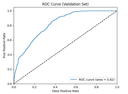
- Quantitative Metrics: The model achieved a Validation Accuracy of 72.6%. The AUC-ROC was 0.82, indicating decent separability.
- Training Dynamics: A notable observation was that the Training Accuracy (~50%) remained lower than Validation Accuracy for several epochs. This confirms that the aggressive data augmentation and dropout successfully prevented memorization, forcing the model to learn robust features that generalized well to the “clean” validation images.
4.1.2. Optimized PyTorch CNN (“MyDeepCNN”)
The transition to the optimized PyTorch pipeline yielded a significant performance boost, validating the effectiveness of the AdamW optimizer and Cosine Annealing scheduler.
- Metrics: This model achieved a Validation Accuracy of 85.9%, a substantial improvement (+13.3%) over the baseline.
- Precision/Recall: It demonstrated high precision (90.8%) with balanced recall (81.9%), resulting in an F1-score of 86.0%.
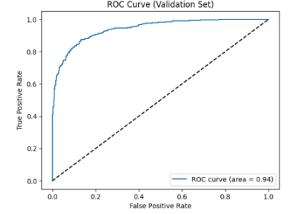
- AUC: The Area Under the Curve reached 0.94, classifying it as an excellent predictor [23].
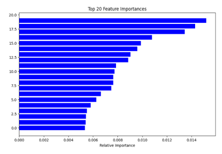
Figure 2: Feature Importance plot extracted from the Random Forest classifier using ResNet50 features.
4.2. Transfer Learning with Classical Classifiers
The feature-based models (ResNet50 + Classical ML) demonstrated the highest overall performance, benefiting from the massive pre-training of the ResNet backbone.
4.2.1. Random Forest (RF)
- The RF classifier achieved a Validation Accuracy of 90.8% and an AUC of 0.97.
- Feature Analysis: The training accuracy was near-perfect (~99.9%), which is characteristic of Random Forests. However, the high validation score proves that this was not detrimental overfitting, but rather a successful mapping of the feature space.
- Feature Importance: Analysis of the decision trees revealed that specific latent features from the ResNet50 vector (e.g., indices corresponding to texture and facial contours) had a disproportionately high impact on the classification decision.
To provide deeper insight into the decision-making mechanism of the ensemble classifier and mitigate the “black-box” nature of deep learning, we conducted a rigorous Feature Importance analysis based on the Mean Decrease in Impurity (MDI) metric. Figure 2 visualizes the relative importance of the top-20 most influential features selected from the 2,048-dimensional embedding vector generated by the ResNet50 backbone.
The disparity in importance scores reveals that the classification capability is not uniformly distributed across all dimensions; rather, the Random Forest successfully isolated a specific subset of high-level semantic descriptors that possess the highest discriminative power. Since these features originate from the final convolutional block of a network pre-trained on ImageNet, the top-ranking dimensions likely correspond to robust latent patterns—such as specific textural details, facial contours, or geometric structures—that correlate strongly with the target classes. This analysis confirms that the ensemble model did not merely memorize training noise but effectively identified and leveraged the underlying semantic structure encoded by the deep network, thereby validating the efficacy of the transfer learning strategy.
4.2.2. Logistic Regression (LR)
- The LR model emerged as the top performer in terms of pure metrics, achieving a Validation Accuracy of 94.8% and a near-perfect AUC of 0.99.
- Interpretation: This result suggests that the 2048-dimensional feature space generated by ResNet50 is linearly separable for the binary face classification task, rendering complex non-linear classifiers unnecessary for this specific feature set.
4.3. Comparative Summary
Table 1 summarizes the performance metrics across all evaluated methodologies. It is evident that while the optimized CNN (MyDeepCNN) provides a strong end-to-end solution, the Transfer Learning approach yields superior accuracy with reduced training complexity.
4.4. Visual Analysis (ROC and Confusion Matrices)
To further validate the statistical significance of our results, we examined the ROC curves and Confusion Matrices.
ROC Curves (Figure 2 & 3): The Receiver Operating Characteristic (ROC) curves illustrate the trade-off between the True Positive Rate (Sensitivity) and False Positive Rate (1-Specificity).
- The Baseline CNN (Figure 2) shows a curve that bows gently towards the top-left corner (AUC=0.82).
- The PyTorch CNN (Figure 3) demonstrates a much sharper “elbow” (AUC=0.94), indicating a superior ability to distinguish between classes with fewer false alarms [24].
4.4.1. Confusion Matrices
- For the Baseline, the matrix reveals a higher number of False Positives, consistent with its lower Precision (67.6%).
- The ResNet50 + LR model produced a matrix with minimal off-diagonal elements, misclassifying less than 5% of the validation samples.
As illustrated in Figure 3, the ROC curve of the Baseline CNN exhibits a moderate area under the curve (AUC = 0.82). The curve’s shape indicates that while the model learns, it struggles to maintain a low false positive rate at higher sensitivity thresholds.
In contrast, the Optimized PyTorch CNN demonstrates superior separability, as evidenced by the sharper ‘elbow’ in its ROC curve shown in Figure 4. With an AUC of 0.94, this model significantly outperforms the baseline, offering a much better trade-off between precision and recall.
Table 1: Comparative Performance Metrics on Validation Set
| Model Architecture | Framework | Val Accuracy | Precision | Recall | F1-Score | AUC-ROC |
|---|---|---|---|---|---|---|
| Baseline CNN | TensorFlow | 72.6% | 67.6% | 79.7% | 73.0% | 0.82 |
| Hybrid CNN + MLP | TensorFlow | 73.3% | 67.4% | 83.2% | 73.0% | 0.82 |
| My Deep CNN (Optimized) | PyTorch | 85.9% | 90.8% | 81.9% | 86.0% | 0.94 |
| ResNet50 + Random Forest | Scikit-Learn | 90.8% | 93.1% | 89.4% | 91.0% | 0.97 |
| ResNet50 + Logistic Regression | Scikit-Learn | 94.8% | 95.0% | 95.3% | 95.0% | 0.99 |
5. Discussion
5.1. Deep Learning: Frameworks and Optimization
A critical finding of this study is the substantial performance gap between the Baseline CNN (TensorFlow) and the Optimized CNN (PyTorch), despite similar architectural depths. The Baseline model achieved 72.6% accuracy, while the Optimized model reached 85.9%. This improvement is attributed to three specific factors:
- Optimization Strategy: The switch from standard Adam to AdamW proved decisive. By decoupling weight decay from gradient updates, AdamW prevented the weights from growing too large without interfering with the adaptive learning rates.
- Learning Rate Scheduling: The Cosine Annealing scheduler allowed the PyTorch model to traverse the loss landscape more effectively, avoiding the local minima where the static learning rate of the Baseline model likely stagnated.
- Activation Functions: The use of LeakyReLU prevented the “dead neuron” issue, maintaining gradient flow throughout the deep network.
5.2. The “Underfitting Paradox” vs. Classical Overfitting
We observed two distinct training behaviors that warrant explanation:
Baseline CNN (Underfitting): As noted in the results, the Baseline CNN exhibited Training Accuracy (~50%) lower than Validation Accuracy (~72%) for initial epochs. This counter-intuitive phenomenon is
- a direct result of the heavy data augmentation and high Dropout (0.5) applied only during training. The model struggles to classify heavily distorted images during training but finds the “clean” validation images easier to classify. This confirms that the model was not memorizing data but learning robust features.
- Classical Models (Overfitting): Conversely, the Random Forest classifier achieved nearly 100% Training Accuracy. While this typically signals overfitting, the high Validation Accuracy (90.8%) indicates that the model successfully captured the underlying structure of the ResNet50 feature space. However, the slightly superior performance of Logistic Regression (94.8%) suggests that the pre-extracted features were already linearly separable, making the complex non-linear decision boundaries of the Random Forest unnecessary.
5.3. Trade-offs: End-to-End vs. Transfer Learning
Our experiments highlight a clear trade-off. Transfer Learning (ResNet50 + LR) offered the highest accuracy (94.8%) with minimal training time (seconds), as it leverages millions of pre-learned parameters. However, it relies on a massive external model (23M parameters). The Optimized CNN, trained from scratch, offers a lighter, self-contained solution (fewer parameters) that still achieves high performance (85.9%), making it suitable for environments where pre-trained models cannot be deployed or where the domain differs significantly from ImageNet.
6. Conclusion
This paper presented a rigorous comparative analysis of binary face classification methodologies. We demonstrated that while training deep CNNs from scratch is challenging due to data scarcity, rigorous optimization (AdamW, Cosine Annealing, Data Augmentation) can yield competitive results. However, the study conclusively shows that Transfer Learning, specifically utilizing ResNet50 features combined with Logistic Regression, provides the optimal balance of accuracy (94.8%) and computational efficiency for this task. The results validate that “off-the-shelf” deep features are robust enough to outperform even carefully tuned custom CNNs in small-to-medium dataset regimes.
6.1. Future Work
Future research will focus on extending these findings in the following directions:
- Dataset Expansion: Evaluating the models on larger, more diverse datasets (e.g., CelebA, LFW) to verify the generalizability of the PyTorch optimization pipeline.
- Advanced Architectures: Investigating modern architectures such as EfficientNetV2 or Vision Transformers (ViT), which may offer better parameter efficiency than ResNet50.
- Ensemble Methods: Creating a voting ensemble that combines the predictions of the Optimized CNN and the Random Forest to potentially push accuracy beyond 95%.
- A. Krizhevsky, I. Sutskever, and G. E. Hinton, “ImageNet classification with deep convolutional neural networks,” in Advances in Neural Information Processing Systems, 2012, pp. 1097–1105. doi:10.1145/3065386.
- K. He, X. Zhang, S. Ren, and J. Sun, “Deep residual learning for image recognition,” in Proceedings of the IEEE conference on computer vision and pattern recognition, 2016, pp. 770–778. doi:10.1109/CVPR.2016.90.
- J. Yosinski, J. Clune, Y. Bengio, and H. Lipson, “How transferable are features in deep neural networks?,” in Advances in neural information processing systems, 2014, pp. 3320–3328. Link: https://proceedings.neurips.cc/paper/2014/file/375c71349b295f059961d99a30030c5e-Paper.pdf
- L. Breiman, “Random Forests,” Machine Learning, vol. 45, no. 1, pp. 5–32, 2001. doi:10.1023/A:1010933404324.
- S. Ioffe and C. Szegedy, “Batch Normalization: Accelerating Deep Network Training by Reducing Internal Covariate Shift,” arXiv preprint arXiv:1502.03167, 2015. doi:10.48550/arXiv.1502.03167.
- M. Tan and Q. V. Le, “EfficientNet: Rethinking Model Scaling for Convolutional Neural Networks,” in International Conference on Machine Learning (ICML), 2019, pp. 6105–6114. Link: https://proceedings.mlr.press/v97/tan19a.html
- S. Yang, W. Xiao, M. Zhang, S. Guo, J. Zhao, and F. Shen, “Image Data Augmentation for Deep Learning: A Survey,” arXiv preprint arXiv:2204.08610, 2023. doi:10.48550/arXiv.2204.08610.
- D. P. Kingma and J. Ba, “Adam: A Method for Stochastic Optimization,” arXiv preprint arXiv:1412.6980, 2014. doi:10.48550/arXiv.1412.6980.
- Kaggle, “Face Classification Dataset,” Kaggle Datasets, [Online]. Available: https://www.kaggle.com/ (Accessed: 2024).
- R. Kohavi, “A study of cross-validation and bootstrap for accuracy estimation and model selection,” in Proceedings of the 14th International Joint Conference on Artificial Intelligence (IJCAI), 1995, vol. 2, pp. 1137–1143. Link: https://www.ijcai.org/Proceedings/95-2/Papers/016.pdf
- Y. LeCun, L. Bottou, G. B. Orr, and K.-R. Müller, “Efficient BackProp,” in Neural Networks: Tricks of the Trade, Springer, 2012, pp. 9–48. doi:10.1007/978-3-642-35289-8_3.
- C. Shorten and T. M. Khoshgoftaar, “A survey on Image Data Augmentation for Deep Learning,” Journal of Big Data, vol. 6, no. 1, p. 60, 2019. doi:10.1186/s40537-019-0197-0.
- L. Perez and J. Wang, “The Effectiveness of Data Augmentation in Image Classification using Deep Learning,” arXiv preprint arXiv:1712.04621, 2017. DOI: doi:10.48550/arXiv.1712.04621.
- M. Abadi et al., “TensorFlow: A System for Large-Scale Machine Learning,” in Proceedings of the 12th USENIX Symposium on Operating Systems Design and Implementation (OSDI), 2016, pp. 265–283. Link: https://www.usenix.org/system/files/conference/osdi16/osdi16-abadi.pdf
- A. Paszke et al., “PyTorch: An Imperative Style, High-Performance Deep Learning Library,” in Advances in Neural Information Processing Systems (NeurIPS), 2019, vol. 32, pp. 8024–8035. Link: https://proceedings.neurips.cc/paper/2019/file/bdbca288fee7f92f2bfa9f7012727740-Paper.pdf
- F. Pedregosa et al., “Scikit-learn: Machine Learning in Python,” Journal of Machine Learning Research, vol. 12, pp. 2825–2830, 2011. Link: https://jmlr.org/papers/v12/pedregosa11a.html
- N. Srivastava, G. Hinton, A. Krizhevsky, I. Sutskever, and R. Salakhutdinov, “Dropout: A Simple Way to Prevent Neural Networks from Overfitting,” The Journal of Machine Learning Research, vol. 15, no. 1, pp. 1929–1958, 2014. Link: https://jmlr.org/papers/v15/srivastava14a.html
- B. Xu, N. Wang, T. Chen, and M. Li, “Empirical Evaluation of Rectified Activations in Convolutional Network,” arXiv preprint arXiv:1505.00853, 2015. doi:10.48550/arXiv.1505.00853.
- I. Loshchilov and F. Hutter, “Decoupled Weight Decay Regularization,” in International Conference on Learning Representations (ICLR), 2019. Link: https://openreview.net/forum?id=Bkg6RiCqY7
- I. Loshchilov and F. Hutter, “SGDR: Stochastic Gradient Descent with Warm Restarts,” in International Conference on Learning Representations (ICLR), 2017. Link: https://openreview.net/forum?id=Skq89Scxx
- A. S. Razavian, H. Azizpour, J. Sullivan, and S. Maki, “CNN Features Off-the-Shelf: An Astounding Baseline for Recognition,” in Proceedings of the IEEE Conference on Computer Vision and Pattern Recognition (CVPR) Workshops, 2014, pp. 806–813. doi:10.1109/CVPRW.2014.122.
- D. W. Hosmer Jr., S. Lemeshow, and R. X. Sturdivant, Applied Logistic Regression, 3rd ed. Hoboken, NJ: Wiley, 2013. doi:10.1002/9781118548387.
- A. P. Bradley, “The use of the area under the ROC curve in the evaluation of machine learning algorithms,” Pattern Recognition, vol. 30, no. 7, pp. 1145–1159, 1997. doi:10.1016/S0031-3203(96)00142-2.
- D. Chicco and G. Jurman, “The advantages of the Matthews correlation coefficient (MCC) over F1 score and accuracy in binary classification evaluation,” BMC Genomics, vol. 21, no. 6, 2020. doi:10.1186/s12864-019-6413-7.