We investigated whether post-hoc calibration improves the trustworthiness of heart-disease risk predictions beyond discrimination metrics. Using a Kaggle heart-disease dataset (n = 1,025), we created a stratified 70/30 train-test split and evaluated six classifiers, Logistic Regression, Support Vector Machine, k-Nearest Neighbors, Naive Bayes, Random Forest, and XGBoost. Discrimination was quantified by stratified 5-fold cross-validation with thresholds chosen by Youden’s J inside the training folds. We assessed probability quality before and after Platt scaling, isotonic regression, and temperature scaling using Brier score, Expected Calibration Error with equal-width and equal-frequency binning, Log Loss, reliability diagrams with Wilson intervals, and Spiegelhalter’s Z and p. Uncertainty was reported with bootstrap 95% confidence intervals, and calibrated versus uncalibrated states were compared with paired permutation tests on fold-matched deltas. Isotonic regression delivered the most consistent improvements in probability quality for Random Forest, XGBoost, Logistic Regression, and Naive Bayes, lowering Brier, ECE, and Log Loss while preserving AUC ROC in cross-validation. Support Vector Machine and k-Nearest Neighbors were best left uncalibrated on these metrics. Temperature scaling altered discrimination and often increased Log Loss in this structured dataset. Sensitivity analysis showed that equal-frequency ECE was systematically smaller than equal-width ECE across model-calibration pairs, while preserving the qualitative ranking of methods. Reliability diagrams built from out-of-fold predictions aligned with the numeric metrics, and Spiegelhalter’s statistics moved toward values consistent with better absolute calibration for the models that benefited from isotonic regression. The study provides a reproducible, leakage-controlled workflow for evaluating and selecting calibration strategies in structured clinical feature data.

1. Introduction

1.1. Background

Heart disease continues to be the major leading cause of death globally. It was recorded that heart disease was responsible for an estimated 19.8 million deaths in 2022 [1]. However, early and accurate prediction plays a significant role in the prevention of adverse results and reduction in healthcare costs. Machine learning (ML) models are increasingly adopted for diagnostic and prognostic tasks in cardiology due to their ability to uncover complex patterns in large clinical datasets [2]. 

Early ML research on heart disease cohorts primarily focused on classification accuracy, with studies routinely reporting performance above 97% using supervised classifiers [3]. These models have the capacity to learn non-linear relationships and high-dimensional interactions between contributing factors such as age, cholesterol, blood pressure, and electrocardiogram results. For example, algorithms such as Random Forest and Gradient Boosting have demonstrated superior performance to identify subtle indicators of cardiovascular abnormalities compared to traditional rule-based systems [4]. This makes them powerful techniques for risk stratification and preventive care.

However, there could be possibility that the models often provide high predictive performance, while probabilistic outputs can be poorly calibrated. That is, the confidence scores they assign do not always align with actual probabilities of disease presence [5]. In high-stakes domains such as healthcare system, well-calibrated predictions are more important to guide the appropriate treatment decisions and manage clinical risks efficiently. Miscalibrated models may lead to overconfident or underconfident decisions, ultimately compromising patient safety [6].  This has prompted a growing interest in uncertainty quantification and post hoc calibration methods, which can adjust the model’s output probabilities without retraining the original model [7]. The importance of these methods has increased in response to an increasing demand for transparent and trustworthy AI systems in clinical settings, particularly with the rise of explainable AI initiatives [8].

Furthermore, recent research has proven that visual tools such as reliability diagrams and calibration metrics such as Expected Calibration Error (ECE), Brier score, and log loss are important in evaluating how well a model is calibrated [9]. While accuracy and AUROC (Area Under the Receiver Operating Characteristic curve) remain popular metrics for model evaluation, they are insufficient for assessing how well a model estimates uncertainty. These metrics provide both quantitative and visual representations of uncertainty and prediction quality, which are vital for gaining the confidence of clinical stakeholders.

1.2. Motivation and Problem Statement

One of the major challenges faced by the medical health sector is the inability to detect early stages of problems related to the heart. When making decisions in the clinical sector, uncalibrated predictions may be misleading. For example, if a model predicts that a patient has a 90% chance of developing heart disease, clinicians must trust that this probability truly reflects clinical reality, otherwise this could lead to incorrect decisions and poor outcomes for the patient.

In many studies, calibration and uncertainty quantification in medical AI systems are often overlooked, leading to a gap between predictive performance and clinical trust [6]. However, this paper addresses that gap by evaluating the calibration of several popular classifiers using post hoc techniques. 

1.3. Scope and Contributions

This study aims to evaluate and compare uncertainty estimation of heart disease prediction models. The research is guided by the following questions:

1. How do post-hoc calibration methods (Platt scaling, temperature scaling and isotonic regression) affect the uncertainty, calibration quality, and prediction confidence of machine learning models for heart disease classification?
2. What are the baseline levels of calibration and uncertainty (ECE, Brier score, log loss, sharpness, Spiegelhalter’s Z-score) for heart disease prediction before and after post-hoc calibration?
3. How does each model (e.g., Random Forest, XGBoost, SVM, KNN and Naive Bayes) perform in terms of probability calibration for heart disease before and after applying post hoc calibration?

Below, we delineate the contributions of this work in light of the research questions above. We conduct a systematic, model-agnostic evaluation of post-hoc calibration for heart-disease prediction, quantifying how Platt (sigmoid) and isotonic mapping alter probability quality without retraining the base models. Beyond headline discrimination metrics, we emphasize clinically relevant probability fidelity, calibration, sharpness, and statistical goodness-of-fit. This study makes four (4) contributions, summarized as follows: 

1. A side-by-side pre/post analysis of six machine learning classifiers using reliability diagrams plus Brier, ECE, log loss, Spiegelhalter’s Z/p, and sharpness to provide complementary views of probability quality for heart disease prediction.
2. Empirical demonstration that isotonic calibration most consistently improves probability estimates, whereas Platt and temperature scaling helps some models but can worsen others. 
3. Despite perfect test-set discrimination for some model, reliability diagrams reveal overconfidence pre-calibration, demonstrating why discrimination alone is insufficient for clinical use.
4. Analysis of variance in predicted probabilities shows calibration-induced smoothing and overconfidence correction, clarifying confidence reliability trade-offs relevant to clinical interpretation.

1.4. Related Works

1.4.1. Machine Learning in Heart Disease Prediction: Calibration and Reliability Considerations 

Machine learning (ML) techniques have been widely applied to predict cardiovascular disease outcomes, typically using patient risk factor data to classify the presence or risk of heart disease. For example, in heart disease prediction using supervised machine learning algorithms: Performance analysis and comparison, [10] evaluated several classifiers (KNN, decision tree, random forest, etc.) on a Kaggle heart disease dataset. They reported perfect performance with random forests achieving 100% accuracy (along with 100% sensitivity and specificity). However, their evaluation emphasized accuracy and did not include any probability calibration or uncertainty quantification. Similarly, [11] evaluation of Heart Disease Prediction Using Machine Learning Methods with Elastic Net Feature Selection compared logistic regression (LR), KNN, SVM, random forest (RF), AdaBoost, artificial neural network (ANN), and multilayer perceptron on the Kaggle dataset used in this study. They found RF to attain ~99% accuracy and AdaBoost ~94% on the full feature set and observed SVM performing best after SMOTE class-balancing and feature selection. Like [10], this study focused on accuracy improvements and other discrimination metrics, with no model calibration applied.

Another work by [12], they also utilized the Kaggle dataset we explored. They evaluated a wide range of classifiers including RF, decision tree (DT), gradient boosting (GBM), KNN, AdaBoost, LR, ANN, QDA, LDA, SVM and reported extremely high accuracy for ensemble methods. In fact, their RF model reached 100% training accuracy (and ~99% under cross-validation). Despite reporting precision, recall, F1-score, and ROC-AUC for each model, this work too did not report any calibration metrics or uncertainty estimates; the focus remained on discrimination performance.

Beyond the popular Kaggle/UCI datasets, researchers have explored ML on other heart disease cohorts. For instance, [13] in A Machine Learning Model for Detection of Coronary Artery Disease applied ML to the Z-Alizadeh Sani dataset (303 patients from Tehran’s Rajaei cardiovascular center). They employed six algorithms (DT, deep neural network, LR, RF, SVM, and XGBoost) to predict coronary artery disease (CAD). After Pearson-correlation feature selection, the best results were achieved by SVM and LR, each attaining 95.45% accuracy with 95.91% sensitivity, 91.66% specificity, F1≈0.969, and AUROC ≈0.98. Notably, although this study achieved excellent discrimination, it did not incorporate any post-hoc probability calibration or uncertainty analysis, the evaluation centered on accuracy and ROC curves alone.

In [14], the authors took a different approach by leveraging larger, real-world data. In an interpretable LightGBM model for predicting coronary heart disease: Enhancing clinical decision-making with machine learning, they trained a LightGBM model on a U.S. CDC survey dataset (BRFSS 2015) and validated on two external cohorts (the Framingham Heart Study and the Z-Alizadeh Sani data). The LightGBM achieved about 90.6% accuracy (AUROC ~81.1%) on the BRFSS training set, with slightly lower performance on Framingham (85% accuracy, ~67% AUROC) and Z-Alizadeh (80% accuracy). While [14] prioritized model interpretability (using SHAP values) and reported standard metrics like accuracy, precision, recall, and AUROC, they did not report any calibration-specific metrics (e.g. no ECE, Brier score, or reliability diagrams), nor did they apply Platt scaling or isotonic regression in their pipeline. Several recent studies have pushed accuracy to very high levels by combining datasets or using advanced ensembles, yet still largely ignore calibration. In [15], the authors proposed a hybrid approach for predicting heart disease using machine learning and an explainable AI method, where they combined a private hospital dataset with a public one and used feature selection plus ensemble methods. Their best model (an XGBoost classifier on a selected feature subset SF-2) achieved 97.57% accuracy with 96.61% sensitivity, 90.48% specificity, 95.00% precision, F1=92.68%, and 98% AUROC. Despite this impressive performance, no probability calibration was mentioned; the study’s contributions focused on maximizing accuracy and explaining feature impacts (via SHAP) rather than assessing prediction uncertainty. 

Using a clinical and biometric dataset (n=571) with a man-in-the-loop paradigm for assessing coronary artery disease, [16] compared standard ML classifiers; best accuracy reached ≈83% with expert input, but the work emphasized explainability over probabilistic calibration. To address the need for diverse and comprehensive research, we conducted a lightweight systematic review and surveyed a range of peer reviewed studies on ML for heart disease prediction in the last 5–10 years with focus on a minimum of 5,000 cohort patients built into the experimental setup. Table 1 summarizes key studies, including their data sources, ML approaches, and whether model calibration was evaluated (and how). Each study is cited with its year and reference number (e.g., 2025 [17] means the study was published in 2025 and is reference [17] in the reference list).

Table 1: Recent ML-based heart disease prediction studies (2017-2025) – Summary of data, methods, and calibration evaluation. (Calibration metrics: HL = Hosmer–Lemeshow test; ECE = Expected Calibration Error; O/E = observed-to-expected ratio; Brier = Brier score.)

1.4.2. Gaps in Research

Despite abundant work on ML-based heart disease prediction, there are clear gaps in the literature regarding probability calibration and uncertainty quantification. First, most studies prioritize discriminative performance (accuracy, F1, AUROC, etc.) and devote little or no attention to how well the predicted probabilities reflect true risk. As shown above, prior works seldom report calibration metrics like ECE or Brier score, nor do they plot reliability diagrams. For example, none of the 10+ studies reviewed applied calibration methods such as Platt scaling or isotonic regression to their classifiers, except for only one study [28]. This indicates a lack of focus on calibration quality, an important aspect if these models are to be used in clinical decision-making where calibrated risk predictions are crucial.

Second, there is a lack of unified evaluation across multiple models and calibration techniques. Prior research typically evaluates a set of ML models on a dataset (as in comparative studies) but stops at reporting raw performance metrics. No study to date has systematically taken multiple classification models for heart disease and evaluated them before and after post-hoc calibration. This means it remains unclear how different algorithms (e.g. an SVM vs. a random forest) compare in terms of probability calibration (not just classification accuracy), and whether simple calibration methods can significantly improve their reliability. Furthermore, the interplay between model uncertainty (e.g. variance in predictions) and calibration has not been explored in this domain. Third, most heart disease prediction papers do not report uncertainty metrics or advanced calibration statistics.  Metrics such as the Brier score (which combines calibration and refinement), the ECE (Expected Calibration Error), or even more domain-specific checks like Spiegelhalter’s Z-test for calibration, are virtually absent from prior studies. Sharpness (the concentration of predictive distributions) and other uncertainty measures are also not discussed. This leaves a research gap in understanding how confident we can be in these model predictions and where they might be over or under-confident. For instance, none of the reviewed studies provide reliability diagrams to visually inspect calibration; as a result, a model claiming 95% accuracy might still make poorly calibrated predictions (overestimating or underestimating risk). 

To the best of our knowledge, no prior work has offered a comprehensive evaluation of pre and post-calibration metrics across multiple models on the specific Kaggle heart disease dataset (1,025 records) used in this study. While several papers have used this or similar data for model comparison, none have examined calibration changes (ECE, log-loss, Brier, sharpness, Spiegelhalter’s Z-test, calibration curves) resulting from post-hoc calibration methods (Platt scaling, isotonic regression). In short, existing studies have left a critical question unanswered: if we calibrate our heart disease prediction models, do their confidence estimates become more trustworthy, and how does this vary by model? Addressing this gap is the focus of our work. We provide a thorough assessment of multiple classifiers before and after calibration, using a suite of calibration and uncertainty metrics not previously applied in this context, thereby advancing the evaluation criteria for heart disease ML models beyond conventional accuracy-based measures. 

2. Materials and Methods

2.1. Research Methodology Overview 

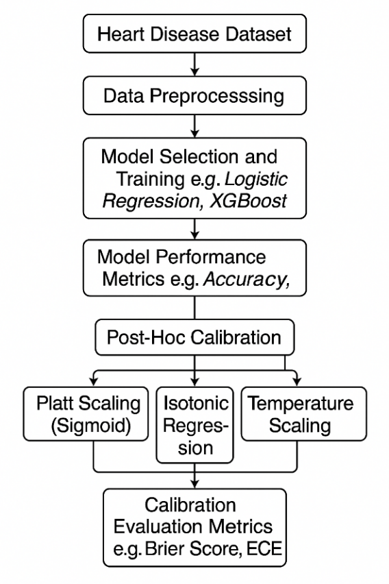
This study employs a structured machine learning workflow to predict heart disease risk based on clinical and demographic variables. As outlined in Figure 1, the process begins with the heart disease dataset, followed by data preprocessing, model selection and training, performance evaluation, and post-hoc calibration. Three (3) calibration techniques (i.e Platt Scaling, Isotonic Regression and Temperature scaling) are applied to refine probabilistic outputs, with effectiveness assessed.

2.2. Description of the Dataset 

The Heart Disease dataset used in this study was sourced from Kaggle. It was originally sourced by merging data from four medical centers Cleveland, Hungary, Switzerland and VA Long Beach, bringing the sample size to 1,025 records, including 713 males (69.6%) and 312 females (30.4%), ages ranging between 29 – 77 years (median age ~56). The dataset contains 14 variables encompassing demographic, clinical and diagnostic test features. Descriptions of the dataset are outlined in Table 2. 

The dataset was inspected for missing values and none was identified. The target variable (heart disease) was approximately balanced, with 51.3% of records labelled Presence of Disease and 48.7% labelled absence of Disease as shown in Figure 2. The target was binarised as heart disease = 1 and absence = 0, retained as an integer. Any re-coding of the target labels was not required for the present analysis.

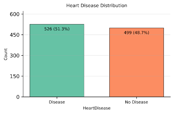
Table 2: Data description for heart disease dataset

2.3. Data Preprocessing 

In this study, the dataset was separated into 13 predictors (i.e patient risk factors) and the 1 outcome feature (i.e the presence or risk of heart disease). Predictors were further divided into two groups: numerical features (e.g Age, RestingBP, Cholesterol) and categorical features (e.g ChestPainType, RestingECG, Thalassemia, Sex). We scale numerical features using a RobustScaler approach, which centres values around the median and spreads them according to the interquartile range. This method was selected due to it being less sensitive to outliers and skewness [30]. For categorical features, a One-Hot Encoding approach was applied, converting each category into binary (0/1) variables. This ensured that all categories were represented in a machine-readable format. 

To prevent information leakage, all preprocessing steps were fit on training data only and were implemented inside the model pipelines. Within each cross-validation fold, imputation, scaling, and encoding were learned on the fold’s training split and then applied to the corresponding validation split. The same rule was followed for the final 70/30 train-test split, where transformers were fit on the 70% training partition and then applied to the held-out 30% test set. Where missing values occurred, numerics were imputed by the median and categoricals by the most frequent level before scaling or encoding. The outcome remained binary as integers throughout the workflow.

2.4. Model Selection

In this work, we benchmark six models (spanning linear, non-linear and ensemble model architectures) to classify patients based on the presence or absence of heart disease. The selected models include Logistic Regression (LR), Support Vector Machines (SVM), Random Forest (RF), Extreme Gradient Boosting (XGBoost), K-Nearest Neighbors (KNN), and Naive Bayes (NB). Using training (70%) and testing (30%) sets, we trained each model on the preprocessed training data and evaluated it on the held-out test data.

Logistic Regression (LR): Logistic Regression is a supervised machine learning model well-suited for binary classification, such as determining the presence or absence of heart disease.  LR calculates the probability of a class (e.g., disease or no disease) by applying a sigmoid function to a weighted sum of predictor variables. Its strengths include simplicity, efficiency, and the ability to interpret coefficients as odds ratios, which is valuable in clinical settings for understanding feature importance and risk factors. Logistic Regression has a proven track record in medical research for risk stratification and is easily calibrated for probability estimation [31].

Support Vector Machines (SVM): Support Vector Machines are powerful, supervised classification models that work by finding the optimal hyperplane that separates classes in the feature space. SVMs excel at handling high-dimensional data and can model nonlinear relationships through kernel tricks, making them highly effective for complex medical datasets. Their ability to maximize the margin between classes reduces the likelihood of misclassification, which is especially useful when distinguishing subtle differences between patients with and without heart disease. SVMs are known for their robustness in real-world clinical prediction tasks [32].

Random Forest (RF): Random Forest is an ensemble algorithm that builds multiple decision trees during training and aggregates their outputs via majority voting for classification. It is especially effective at capturing nonlinear relationships and interactions among risk factors in heart disease prediction. The ensemble nature of RF mitigates overfitting and variance, providing more reliable and stable predictions on diverse patient populations. Its embedded feature importance scores help clinicians identify key predictors of heart disease, further supporting its use in healthcare analytics [33].

Extreme Gradient Boosting (XGBoost): XGBoost is a gradient boosting framework that creates a series of weak learners (usually decision trees) and optimizes them sequentially. It is renowned for combining high predictive accuracy with speed and efficiency, making it a top performer in medical classification challenges. XGBoost handles missing data gracefully and is robust to outliers, both of which are common in clinical datasets. Its sophisticated regularization techniques reduce overfitting, and its model interpretability tools are advantageous for validating results in heart disease risk prediction [34].

K-Nearest Neighbors (KNN): K-Nearest Neighbors is a non-parametric classification method that predicts the class of a sample based on the majority class among its k closest neighbors in feature space. KNN is intuitive, easy to implement, and doesn’t assume data distribution, making it suitable for heterogeneous clinical datasets. KNN is effective at leveraging local patterns, which can help identify at-risk heart disease patients by matching them to previously observed cases. However, it can be sensitive to feature scaling and less efficient with extensive datasets [35].

Naive Bayes (NB): Naive Bayes is a probabilistic classification algorithm that applies Bayes’ theorem, assuming feature independence. Its simplicity and computational efficiency make it attractive for medical tasks with many categorical variables. Despite its “naive” independence assumption, NB often performs surprisingly well for heart disease prediction because it can handle missing values, is robust with noisy data, and quickly estimates posterior probabilities. This makes it valuable for real-time risk assessment and decision support in clinical environments [36].

2.5. Model Tuning Strategy

In this study, GridSearchCV was used as the primary hyperparameter-tuning strategy due to its structured and reproducible approach [37], [38]. GridSearchCV works by exhaustively evaluating all possible combinations of predefined hyperparameters for a given algorithm [37], [38]. For each candidate configuration, the model is trained and validated using 5-fold cross-validation, ensuring stable performance estimates; this setup is widely recommended for clinical prediction models and has been applied to heart-disease prediction tasks [39], [40]. This is particularly important in healthcare datasets such as heart disease prediction, where sample sizes may be limited and class distributions may be imbalanced [40], [41]. By systematically exploring the parameter space, GridSearchCV helps identify the configuration that yields an appropriate balance between accuracy and generalisation performance [37], [38], [39]. In our heart-disease model, we used GridSearchCV to improve the stability of probability outputs before applying post-hoc calibration techniques. Table 3 summarises the parameter grid and chosen parameters for each model trained in this experiment.

2.6. Cross-validated discrimination

To measure discrimination outside one held-out test split, we used stratified 5-fold cross-validation on the 70% training set. In every outer fold, the full preprocessing pipeline and the classifier were fitted only on that fold’s training partition, then applied to the corresponding validation partition. This guards against information leakage from scaling or encoding into validation data.

Threshold-dependent metrics used a single, data-driven cutpoint per model based on Youden’s J index. For a given threshold t_on predicted probabilities, J(t) = Sensitivity(t) + Specificity (t) – 1 and the selected cut point is t = arg max t J(t), [42]. Within each outer-fold training partition we ran an inner 5-fold CV to estimate t using only the inner validation predictions, then fixed t and applied it to the outer-fold validation data to compute Accuracy and F1. AUC ROC was computed from continuous scores and did not use a threshold. Using J focuses the operating point where both sensitivity and specificity are jointly maximized in the training data, a practice with well-studied statistical properties for cutpoint selection [43].

Table 3: Hyperparameter Grids and Selected Best Settings by Model

This nested procedure helps control overfitting and preserves statistical validity. The threshold is chosen strictly inside the training portion of each outer fold, never on the outer validation or test data, which avoids optimistic bias and the circularity that arises when model selection and error estimation are performed on the same data [44]. When comparing uncalibrated and calibrated variants, the identical t learned within the outer-fold training data was applied to both sets of probabilities for that fold. This preserves a paired design, reduces variance in fold differences and maintains the validity of subsequent significance testing based on matched resamples [45].

2.7. Model Performance Metrics

We evaluated classification performance using Accuracy, ROC-AUC, Precision, Recall, and F1-score. Let TP, FP, TN, and FN denote true positives, false positives, true negatives, and false negatives, respectively.

Accuracy. Defined as \(\left(\frac{TP+TN}{TP+FP+TN+FN}\right)\), accuracy reflects the share of correctly classified cases in the test set. In clinical screening contexts where disease prevalence may be low accuracy depends on the decision threshold and can mask deficiencies under class imbalance, yielding seemingly strong performance while missing many positive cases [46].

ROC-AUC. The receiver-operating-characteristic area summarizes discrimination across all thresholds; it equals the probability that a randomly selected positive receives a higher score than a randomly selected negative and ranges from 0.5 (no discrimination) to 1.0 (perfect). ROC-AUC is broadly used in clinical prediction for its threshold-agnostic view of separability, though it does not reflect calibration or the clinical costs of specific error types [47].

Precision. Given by \(\left(\frac{TP}{TP+FP}\right)\), quantifies how reliable positive alerts are among patients flagged as having heart disease, the fraction truly positive. As thresholds are lowered to capture more cases, precision typically decreases, illustrating the trade-off clinicians face between false alarms and case finding [48].

Recall. Defined as \(\left(\frac{TP}{TP+FN}\right)\), measures the proportion of truly diseased patients the model detects (sensitivity). Raising recall generally requires a lower threshold, which increases false positives and reduces precision; selecting an operating point should therefore reflect clinical consequences and disease prevalence [49].

F1-score. The harmonic mean \(\left(\frac{\text{Precision}\times\text{Recall}}{\text{Precision}+\text{Recall}}\right)\times 2\), provides a single summary when both missed cases and false alarms matter. F1 is commonly reported in imbalanced biomedical tasks, though its interpretation should be complemented by other metrics given known limitations under skewed prevalence [50].

These metrics establish a consistent baseline for cross-model comparison and inform our subsequent calibration and uncertainty quantification analysis.

2.8. Post-Hoc Calibration and Evaluation

2.8.1. Selected Calibration Techniques

Post-hoc calibration refers to techniques applied after model training that map raw scores to probabilities without changing the underlying classifier. In clinical settings where decisions hinge on risk estimates, these procedures use a held-out calibration set to fit a simple, typically monotonic mapping so that predicted probabilities better match observed event rates [9], [51], [52]. In this study, calibration was fit strictly on training-only validation data inside cross-validation and applied to the corresponding validation folds, then to the held-out test split, which avoids information leakage and optimistic bias as recommended in prior work [5], [7], [9], [51]. 

In clinical text or imaging pipelines for heart-disease prediction, this is attractive, one can retain the trained model and its operating characteristics, then calibrate its outputs to yield probabilities that are more trustworthy for downstream decision thresholds, alerts, or shared decision-making [51], [52]. For this study, we applied three post-hoc calibration methods, Platt scaling, isotonic regression, and temperature scaling, to adjust model outputs into well-calibrated probabilities [5], [7].

• Platt scaling works by fitting a smooth S-shaped sigmoid curve to the model’s scores using a separate validation set, so that predicted probabilities better match actual outcomes. This method is simple and efficient but assumes that the relationship between scores and probabilities follows a logistic pattern [9], [53]. In our pipeline, the sigmoid mapping was learned on training-only validation folds and then applied to their matched validation sets.
• Isotonic regression is a more flexible, non-parametric method that does not assume any specific shape. Instead, it fits a step-like monotonic curve that can adapt to complex patterns in the data [54]. While this flexibility can better capture irregular relationships, it can also lead to overfitting if the validation dataset is small, hence our use of cross-validated, training-only fits to mitigate instability [5], [7], [51].
• Temperature scaling applies a single global temperature T > 0 to sharpen or soften probabilities via p_T = σ (logit(p)/T). We estimated T on training-only out-of-fold predictions by minimizing negative log loss, then applied the learned T to the corresponding validation folds and the held-out test split. Temperature scaling is lightweight and widely used to correct overconfident scores without altering class ranking [5].

In practice, Platt scaling is most useful when a sigmoid relationship is expected, isotonic regression is preferred when the calibration pattern is unknown or more complex [9], and temperature scaling provides a simple, global adjustment of confidence that can be effective when miscalibration is primarily due to score overconfidence rather than shape distortions [5]. Using all three methods provides a robust calibration toolbox, ensuring reliable probability estimates across different models, while our training-only fitting approach addresses concerns about leakage and preserves valid evaluation.

2.8.2. Model Uncertainty Quantification and Calibration Evaluation Metrics

In this study, we measure the uncertainty of the models using these key calibration evaluation metrics: Reliability diagram, Brier Score, Expected Calibration Error (ECE), Log Loss and Sharpness. A combination of these metrics provides a holistic understanding of each model’s effectiveness in quantifying model uncertainty.

Reliability diagram, calibration plot. A reliability diagram visualizes how predicted probabilities align with observed event rates by plotting, across confidence bins, the empirical outcome frequency against the mean predicted probability. A perfectly calibrated model traces the 45-degree diagonal line, while systematic deviations reveal over or under-confidence [9]. Reliability diagrams are standard in forecast verification and machine-learning calibration, and they provide a visual check of probability accuracy while preserving discrimination. Practical caveats include sensitivity to binning and sample size, and the fact that the plot alone does not indicate how many samples fall into each bin, often addressed by adding a companion confidence histogram [5], [55], [56]. We experiment with two binning strategies (i.e equal-width bins and equal-frequency bins). A rolling-mean curve over the predicted probabilities was added to stabilise visual trends without changing the bin statistics.

Brier Score – The Brier Score measures the mean squared difference between predicted probabilities and the actual binary outcomes. Unlike accuracy which reduces predictions to “yes/no” and ignores the uncertainty behind probability values the Brier Score penalizes poorly calibrated or overly confident predictions. This makes it more informative for model uncertainty quantification, especially in clinical settings were knowing the probability of heart disease (and not just a binary label) aids risk discussions and decision-making. Lower Brier Scores indicate better calibrated and more reliable probability forecasts, a key aspect of clinical utility [57].

Expected Calibration Error (ECE). ECE summarizes how closely a model’s predicted probabilities match the observed frequencies of outcomes. It divides predictions into probability bins and measures the mismatch between average predicted probability and the actual outcome rate in each bin. In heart disease prediction, ECE helps verify if model confidence reflects real-world risks, ensuring patients with a predicted 70% heart disease risk, for example, actually face that risk. Lower ECE values indicate better calibrated models, which is crucial for trusted clinical decision support [5]. In this work, we report two ECE variants to assess robustness to binning: equal-width bins with K = 10 and equal-frequency bins with K = 10; the latter balances counts per bin and often yields more stable estimates on modest sample sizes [5], [56].

Log Loss – Log Loss (or cross-entropy loss) evaluates the uncertainty of probabilistic outputs by heavily penalizing confident but incorrect predictions.  Log Loss is sensitive to how far predicted probabilities diverge from the actual class, providing a continuous measure of model reliability. For heart disease prediction, low Log Loss means the model rarely makes wildly overconfident errors, promoting safer, uncertainty-aware clinical interpretation [58].

Sharpness (variance of predicted probabilities) – Sharpness measures the spread or concentration of predicted probabilities, independent of whether they’re correct. High sharpness means the model often predicts risks near 0 or 1, indicating confident, decisive forecasts. For heart disease prediction, greater sharpness is desirable only if paired with good calibration confident predictions should be correct. Thus, sharpness reveals how much intrinsic uncertainty the model expresses, helping physicians judge whether predictions are actionable or too vague for clinical use [55].

Table 4: Pipeline decisions for Baseline Classification Performance & Calibration – summary of experiment setup, evaluation choices, and preprocessing decisions

2.9. Confidence intervals and statistical tests

Confidence intervals. For test-set discrimination metrics, we computed 95% bootstrap percentile intervals with 2,000 resamples, using stratified resampling to preserve class balance and skipping resamples with a single class for AUROC [59]. For cross-validated summaries we formed per-fold estimates, then bootstrapped across the out-of-fold units to obtain fold-aware 95% intervals for Brier score, ECE, Log Loss, and sharpness. For reliability diagrams we reported Wilson 95% intervals for bin-wise observed event rates to stabilize proportions in modest bin counts [60].

Spiegelhalter’s Z-score & p-value – Spiegelhalter’s Z-score tests overall calibration by comparing predicted probabilities to actual outcomes, normalized by their variance. A non-significant p-value suggests the model is well-calibrated; otherwise, the probabilistic forecasts may be systematically over or under-confident. This calibration test is especially important in health applications, assuring clinicians that model probabilities are statistically valid reflections of true outcome chances [61].

Permutation p-tests on fold-matched deltas. To compare calibrated to uncalibrated states we used paired permutation tests on fold-matched differences, for example Δ = metric_cal – metric_uncal​. Within each model, we repeatedly flipped the signs of fold-level deltas to generate the null distribution that the median delta equals zero, using 10,000 permutations, two sided. We report the observed delta, its bootstrap 95% interval, and the corresponding permutation p-value, which answers whether the improvement is larger than expected by chance under the paired design [62], [63].

Wilcoxon signed-rank tests. For the equal-width versus equal-frequency ECE comparison, we also report paired Wilcoxon signed-rank tests on fold-matched differences, alongside bootstrap intervals for the median delta, to summarize direction and robustness of the binning effect without distributional assumptions [64].

3. Baseline model performance

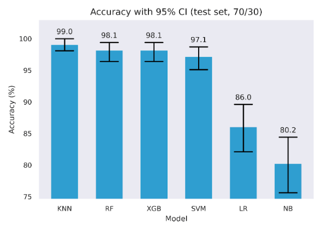
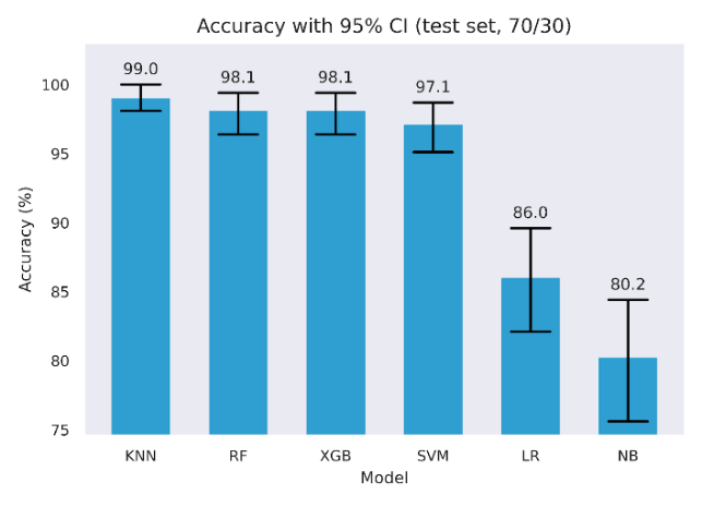
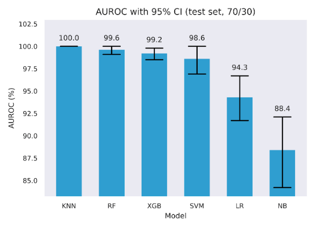
Six classifiers were trained and evaluated on the held-out test set. Table 5 reports Accuracy, F1, and ROC AUC with 95% bootstrap confidence intervals alongside precision and recall. Four models achieved very high scores across metrics, with KNN, Random Forest, XGBoost, and SVM, each reaching high test scores. For example, KNN achieved 99.0% Accuracy, 99.0% F1, and 100.0% ROC AUC, while Random Forest, XGBoost, and SVM were in the 97.1% to 99.6% range across these metrics. Logistic Regression was lower, with 86.0% Accuracy, 86.6% F1, and 94.3% ROC AUC. Naive Bayes was lowest, with 80.2% Accuracy, 77.8% F1, and 88.4% ROC AUC. Confidence intervals are tight for the top four models, as shown in Figures 3 to 5 and wider for Logistic Regression and Naive Bayes, indicating greater sampling uncertainty for the latter pair.

Table 5: Performance metrics of baseline classification models (before calibration) with 95% confidence interval (CI) bootstrap
 (number of boots = 2,000)

To quantify discrimination metric without relying on a single partition, we used stratified 5-fold cross-validation, fitting preprocessing and models within each training fold. We selected the decision threshold by Youden’s J using inner cross-validation, then applied that fixed threshold to the outer validation fold. Following best practice, we tuned the decision threshold in each fold on the training predictions, selecting the cut-point that maximized Youden’s J, rather than using a fixed 0.5 threshold [65], while still maintaining statistical significance [66]. Table 6 reports the fold means for Accuracy, F1, and ROC AUC for the uncalibrated models optimized via Youden J, side by side with baseline performance from Table 5.

Discrimination was strongest for four models, with consistently high values. Random Forest and KNN reach 99.60% Accuracy and 99.60% F1, with ROC AUC at 100.00%. SVM attains 99.0% Accuracy, 99.1% F1, and 100% ROC AUC. XGBoost follows closely with 99.0% Accuracy, 99.0% F1, and 100% ROC AUC. Logistic Regression and Naive Bayes remain well below this cluster, with 86.8% and 83.8% Accuracy, 87.5% and 84.7% F1, and 94.0% and 89.5% ROC AUC, respectively.

These results reflect two effects. First, ROC AUC values confirm very strong class separability on this dataset. Second, optimizing the threshold on training data via Youden’s J raises fold-wise Accuracy and F1 compared with a fixed cutpoint, which explains the higher values relative to our earlier fixed-threshold point estimate summaries [67]. The Youden J optimised values in Table 6 serve as the discrimination baseline for all later comparisons, where we examine how post-hoc calibration changes calibration metrics while tracking any movement in Accuracy and F1 relative to these uncalibrated, Youden-J estimates.

Table 6: Uncalibrated Cross-validated Accuracy, F1, and ROC AUC with tuned parameters

3.1. Reliability Plots

We plot reliability diagrams to visualise calibration effects using out-of-fold predictions from stratified 5-fold cross-validation. Given a test set of 306 instances (30% of the 1,025-record dataset), predicted probabilities were partitioned into ten equal-frequency bins so each bin contained a similar number of cases, which stabilizes bin estimates. This choice balances resolution and stability in modest samples, consistent with guidance that discourages aggressive binning when counts per bin become small [56]. For each bin we plot the bin mean against the observed event rate with Wilson 95% intervals with a thin rolling mean over the sorted predictions. Figures 6 to 9 present the six models for the uncalibrated outputs and for Platt, Isotonic, and Temperature calibration.

Before calibration (Figure 6), Logistic Regression and XGBoost track the diagonal closely through most of the probability range, with small departures near the extremes. Random Forest shows overconfidence in the upper tail, where predicted risks exceed observed frequencies. SVM tracks the diagonal in the mid-range but is less reliable at the extremes. KNN exhibits a flat, underconfident shape over much of the scale. Naive Bayes displays the familiar S-shape, underestimating risk at intermediate probabilities and overshooting near 1, consistent with prior reports of miscalibration for these families of models [7], [9], [53].

Platt scaling (Figure 7) improves Logistic Regression, SVM and Naive Bayes, drawing curves toward the diagonal where deviations were approximately monotonic, but it leaves clear residual error for Random Forest and KNN, likely due to its monotonic, logistic-form constraint [68][69]. XGBoost shows little gain and, in places, mild distortion relative to its already good pre-calibration fit.

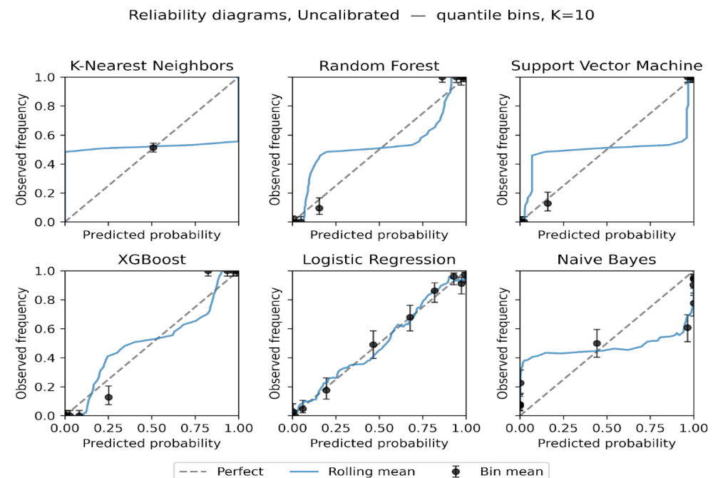
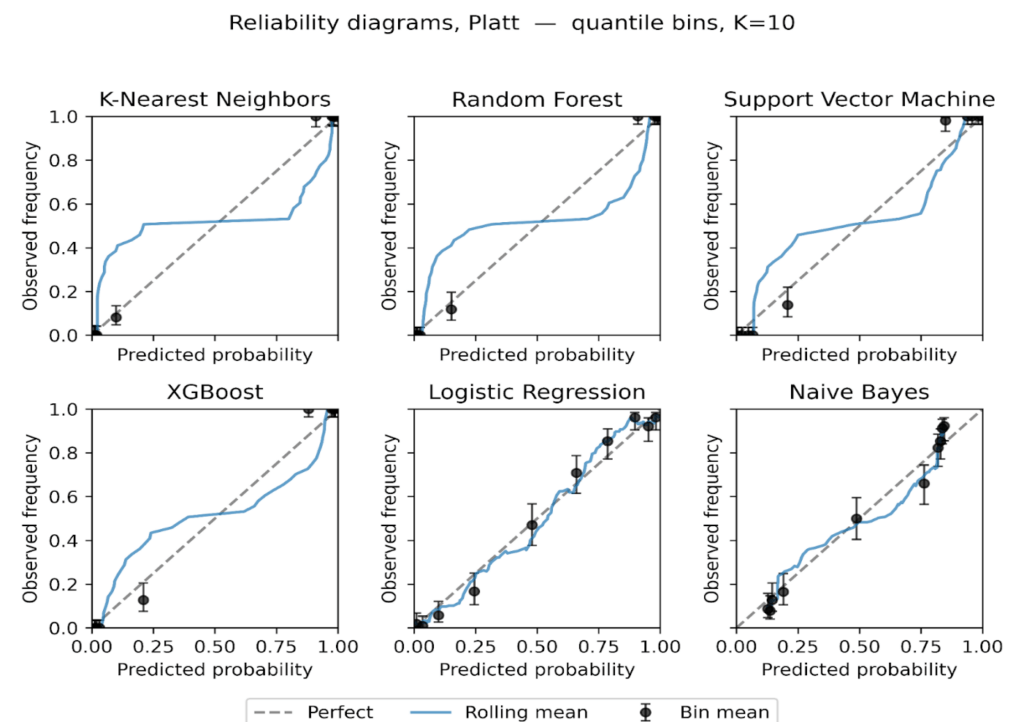
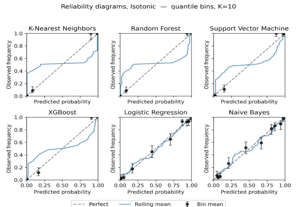
Figure 8: Reliability diagrams after Isotonic regression, equal-frequency bins K = 10.

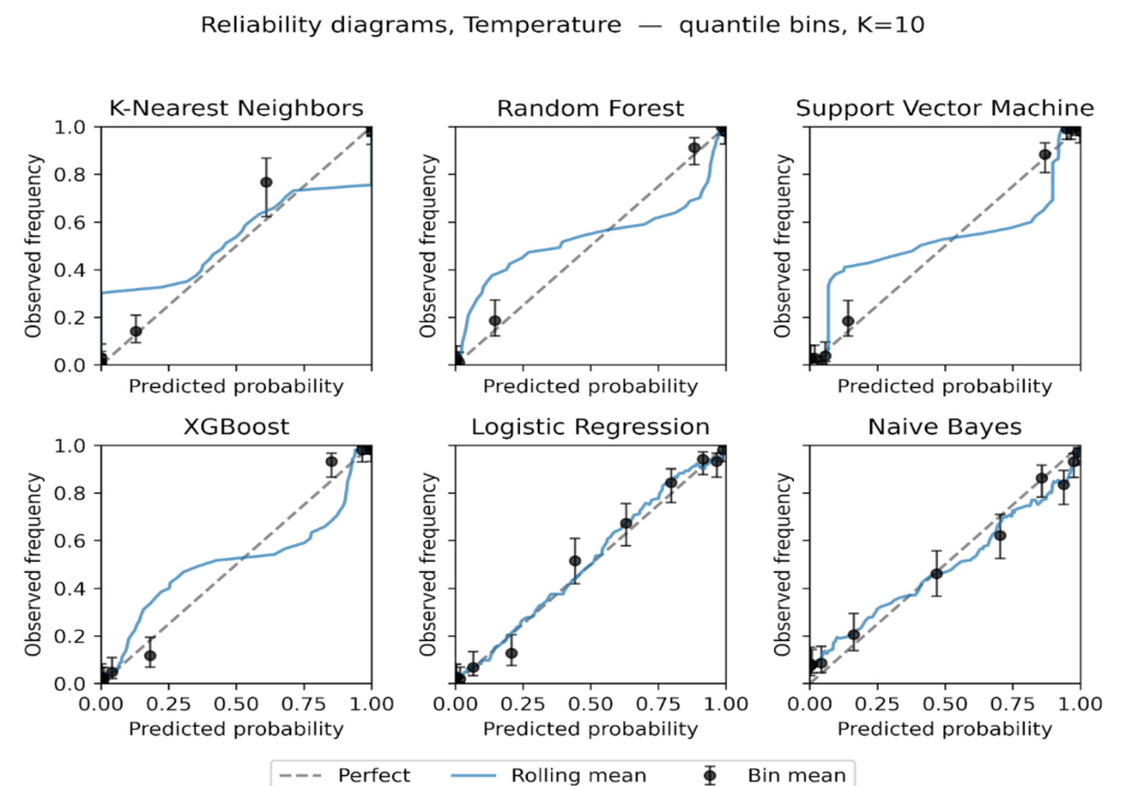
Figure 9: Reliability diagrams after Temperature scaling, equal-frequency bins K = 10.

Isotonic regression (Figure 8) provides the largest and most consistent improvements. Naive Bayes becomes markedly more tightly positioned across the range, and SVM tightens around the diagonal with narrower uncertainty bands. Random Forest is corrected at high probabilities, reducing overconfidence. KNN remains relatively unstable, with small bins at the extremes still showing variance. These findings suggest that while sigmoid calibration is suitable for models with nearly linear miscalibration, isotonic regression better handles complex, non-monotonic distortions in probabilistic estimates [70], [71]. 

Temperature scaling (Figure 9) yields modest, mostly uniform shifts in confidence. It reduces the top-end overconfidence for Random Forest and XGBoost, but its effect is smaller than isotonic and, as expected for a single-parameter rescaling, it does not correct non-linear distortions.

The reliability plots show three consistent themes. First, calibration needs are model-specific, with ensembles tending to be overconfident near 1, Naive Bayes showing S-shaped error, and Logistic Regression close to calibrated at baseline. Second, isotonic is the most effective general-purpose post-hoc adjustment on this dataset, while Platt helps when deviations are nearly logistic in form. Third, confidence intervals make departures from perfect calibration most apparent at the extremes of the probability scale, where data are sparse. 

3.2. Sensitivity of ECE to binning choice

We assessed the stability of ECE using two binning strategies with K = 10, equal-width and equal-frequency. For each model, calibration state, and fold, we computed the paired difference [ΔECE = ECE {_uniform} – ECE {_quantile}]. Positive values indicate smaller ECE when bins carry similar counts. The paired summaries are presented in Table 7 below, and we plot per-model medians with 95 % CIs in Figure 10.

Across all models and calibration states combined, equal-frequency binning produced smaller ECE values. As shown in Table 7, the overall median ΔECE was 0.0069 with a 95 % CI 0.0056 to 0.0089 and a Wilcoxon p value 4.87×10⁻⁸, with 74.2% of paired fold comparisons favoring equal frequency. The largest effects occur for the tree-based ensembles. For XGBoost the median ΔECE was 0.0115 (95 % CI 0.0074 to 0.0149, p 9.54×10⁻⁶), and for Random Forest it was 0.0098 (95 % CI 0.0057 to 0.0119, p 2.61×10⁻⁴). These two bars are the tallest in Figure 10, matching the entries in Table 7.

Table 7: Paired comparison of ECE with K = 10 using equal-width and equal-frequency bins over CV folds. CIs are 95% CIs bootstrap (number of boots = 10,000). Paired Wilcoxon tests on fold-matched deltas.

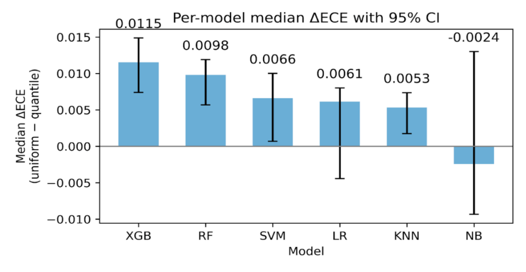
Figure 10: Per-model median ΔECE with 95 % CIs bootstrap (number of boots = 10,000).

SVM and KNN show smaller but consistent gains. As seen in Table 7, SVM has median ΔECE 0.0066 (95 % CI 0.0007 to 0.0100, p 9.44×10⁻³), and KNN has 0.0053 (95 % CI 0.0017 to 0.0074, p 6.55×10⁻⁴). Logistic Regression shows a modest median with a CI that crosses zero, 0.0061 (95 % CI -0.0044 to 0.0080, p 0.277). Naive Bayes shows no advantage for equal-frequency, -0.0024 (95 % CI -0.0093 to 0.0130, p 0.784). These patterns are visible in Figure 10, where LR has a short bar with wide whiskers and NB dips slightly below zero.

By calibration method, the same direction holds. As shown in Table 7, the median ΔECE is 0.0069 for Uncalibrated (95 % CI 0.0012 to 0.0119, p 8.09×10⁻⁵), 0.0068 for Isotonic (95 % CI 0.0048 to 0.0083, p 7.30×10⁻⁴), and 0.0064 for Temperature (95 % CI 0.0004 to 0.0147, p 5.38×10⁻³). Platt shows a positive median 0.0073 with a non-significant p value 0.253, which is consistent with its shorter bar and wide CI in Figure 10.

This sensitivity analysis indicates that ECE is lower on average with equal-frequency bins, as shown in Table 7 and Figure 10. We therefore report both ECE variants throughout and treat the quantile-based ECE as a robustness check rather than as evidence of intrinsically better calibration.

3.3. Calibration metrics by model and calibration method

Table 8 reports fold means for Accuracy, F1, AUC ROC, Brier score, ECE with equal-width bins at K = 10, ECE with equal-frequency bins at K = 10, and Log Loss for each model under Uncalibrated, Platt, Isotonic, and Temperature. We identify the best calibration per model using the rule “best” equals the minimum Brier, the minimum of each ECE variant, and the minimum Log Loss.

Across models, Isotonic most often provides the strongest calibration. This pattern is consistent with the reliability plots where a monotone nonparametric map aligns S-shaped or overconfident regions while preserving ordering. Platt is competitive when deviations are close to a logistic shift, and Temperature yields smaller, uniform corrections that can trim overconfidence without altering rank.

Two models, KNN and SVM, are best uncalibrated across the calibration metrics in this dataset. For these models, applying Platt, Isotonic, or Temperature does not improve Brier, ECE, or Log Loss relative to the uncalibrated scores in Table 8, and in places calibration slightly worsens these quantities. This matches the reliability plots, which show limited systematic miscalibration for SVM and persistent variance for KNN that calibration does not correct.

Table 8: Cross-validated means for Accuracy, F1, AUC ROC, Brier, ECE (uniform, 10), ECE (quantile, 10), and Log Loss by model and calibration method. Bold, per model, the method achieving the minimum for Brier, each ECE variant, and Log Loss.

Random Forest shows its clearest gains under Isotonic. Brier, both ECE variants, and Log Loss are lowest with Isotonic, mirroring the correction of high-probability overconfidence seen in the reliability plots. Accuracy and F1 remain close to the uncalibrated Youden-J values, and AUC ROC is essentially unchanged. XGBoost starts close to calibrated. Differences among methods are small, with Isotonic producing the best Log Loss and competitive ECE values. Accuracy and F1 shift only marginally relative to the uncalibrated Youden-J baseline. Logistic Regression is already well behaved.  Isotonic yields the best Log Loss, ECE, with discrimination metrics essentially unchanged. Naive Bayes shows the largest calibration gains with Isotonic. Brier, both ECE variants, and Log Loss drop, consistent with the straightening of the S-shaped reliability curve. AUC ROC remains constant, and Accuracy and F1 may change slightly without a systematic direction.

On the calibration-discrimination balance, Temperature does not behave as neutral. In your fold means, Temperature shifts Accuracy and F1 for every model, and AUC ROC also changes rather than remaining fixed. Isotonic and Platt tend to preserve AUC ROC within small deltas while improving Brier, ECE, and Log Loss, but Temperature’s global rescaling can move operating points and ranking enough to register in discrimination metrics. Consequently, when discrimination stability is a priority, Isotonic is generally preferred for RF, XGB, LR, and NB, Uncalibrated is preferred for SVM and KNN, and Temperature should be used with caution because of its measurable impact on Accuracy, F1, and sometimes AUC ROC as reflected in Table 8.

3.4. Calibration metrics with uncertainty

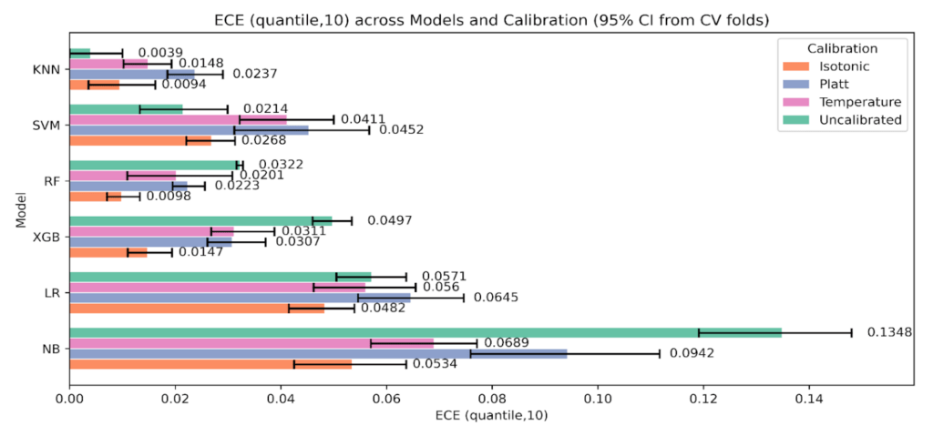
We report cross-validated calibration performance for Uncalibrated, Platt, Isotonic, and Temperature using Brier score, ECE with equal-width bins, K = 10, ECE with equal-frequency bins, K = 10, and Log Loss. Table 9 presents per-model means with 95% bootstrap CIs across folds. These tabulated intervals anchor the comparisons that follow and are the source for the error bars in the grouped plots.

Table 9: Calibration metrics with 95% bootstrap confidence intervals by model and calibration state, number of boots = 2000 

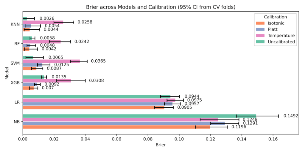
As shown in Figure 11, Brier score with 95% CIs, tree ensembles benefit the most from Isotonic. For Random Forest, Brier drops from 0.0058 uncalibrated to 0.0042 with Isotonic, while Platt and Temperature are higher at 0.0048 and 0.0242. For XGBoost, Brier improves from 0.0135 uncalibrated to 0.0070 with Isotonic, with Platt 0.0092 and Temperature 0.0308. Naive Bayes shows a large reduction relative to its baseline, 0.1492 uncalibrated to 0.1196 with Isotonic. Support Vector Machine and K-Nearest Neighbors are best Uncalibrated on Brier at 0.0065 and 0.0026 respectively, and Temperature is the worst state for both.

Turning to Figure 12, ECE (equal-width, K = 10), Random Forest falls from 0.0449 uncalibrated to 0.0144 with Isotonic, and XGBoost from 0.0639 to 0.0241. Naive Bayes improves from 0.146 to the 0.055-0.062 range under Platt or Isotonic. KNN is already very low uncalibrated at 0.0039, and all calibrators increase uniform-ECE. SVM shows mixed behavior, with Temperature giving a lower uniform-ECE than Platt, yet Brier and Log Loss still favor the uncalibrated state.

The sensitivity of ECE to the binning approach is clear in Figure 13, ECE (equal-frequency, K = 10). Absolute values are smaller and intervals are tighter because bins carry similar counts. Random Forest improves from 0.0322 (uncalibrated) to 0.0098 with Isotonic, and XGBoost improves from 0.0497 to 0.0147. Naive Bayes drops from 0.1348 to 0.0534 with Isotonic, while Platt sits near 0.0942. KNN remains best uncalibrated at 0.0039, with Isotonic 0.0094 and Temperature 0.0148 above that. SVM is lowest Uncalibrated at 0.0214 and rises under calibration, Isotonic 0.0268, Temperature 0.0411, Platt 0.0452.

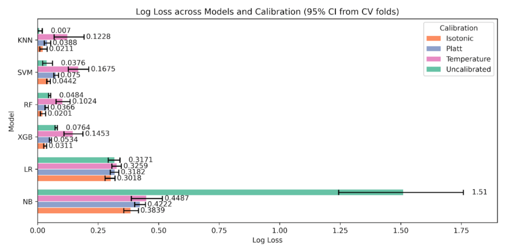
Likelihood trends in Figure 14, Log Loss with 95% CIs, reinforce the Brier score pattern with Temperature worsening on most of the models. Random Forest moves from 0.0484 uncalibrated to 0.0201 with Isotonic. XGBoost drops from 0.0764 to 0.0311. Naive Bayes is most erratic, 1.51 uncalibrated to 0.3839 with Isotonic and 0.4222 with Platt. KNN and SVM are best Uncalibrated at 0.0070 and 0.0376; Temperature increases loss across models. Logistic Regression improves modestly, 0.3171 uncalibrated to 0.3018 with Isotonic.

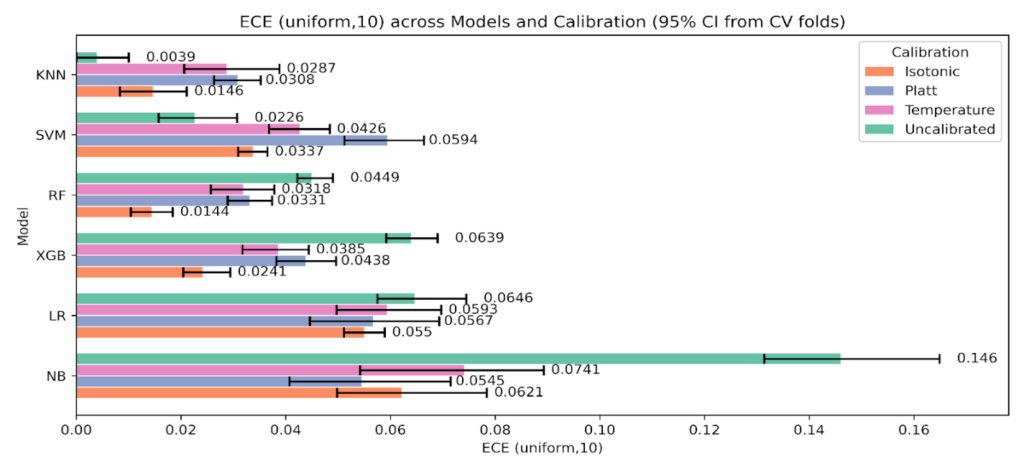
Figure 12: Expected Calibration Error with equal-width bins, K = 10, across models and calibration states with 95% CIs.

The statistical check in Figure 15, Spiegelhalter’s Z and p, complements the aggregate metrics. Values near Z = 0 with p > 0.05 indicate no detectable miscalibration at fold scale. Random Forest stays near zero across states with p ≈ 0.50-0.65, and XGBoost shows Z ≈ 0.25-0.71 with p ≈ 0.40-0.81. Naive Bayes improves from Z = -3.14, p = 0.234 uncalibrated to Z ≈ -0.08 to -0.18 with p ≈ 0.54-0.69 after calibration, consistent with its large reductions in Brier and Log Loss. KNN sits around Z ≈ 0.66-1.05 with p ≈ 0.39-0.66, which matches its already strong Brier and Log Loss when uncalibrated and the lack of benefit from calibration. SVM shows Z ≈ 0.02-0.67 and p ≈ 0.38-0.56, again echoing the mixed ECE behavior and the preference for the uncalibrated state. Logistic Regression remains close to zero, Z from -0.16 to 0.41 with p ≈ 0.49-0.68, in line with small but consistent gains under Isotonic.

We further conducted a statistical comparison test using permutation P-values between pre and post-calibration metrics, setting the number of permutations to 20,000 and the number of bootstraps to 2,000. Table 10 reports changes calculated as calibrated minus uncalibrated for each metric, where negative deltas indicate improvement, with permutation p-values computed on fold-matched resamples.

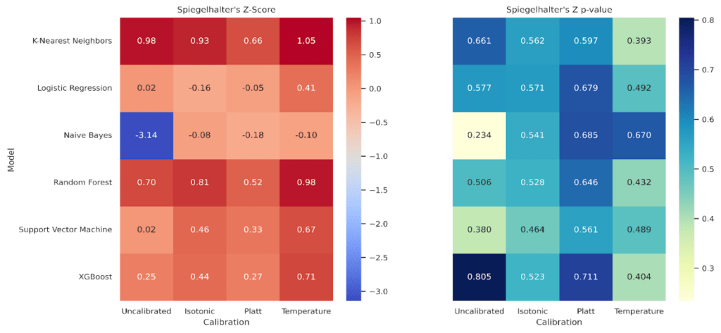
Table 10: Statistical comparison tests using Permutation P between pre and post-calibration metrics.

For Random Forest, Isotonic delivers coherent gains across all metrics, for example ECE with equal-width bins falls by 0.0305 and ECE with equal-frequency bins by 0.0224 with p about 0.06, and Log Loss drops by 0.0283 with similar uncertainty.XGBoost shows the same direction with larger magnitudes, ECE with equal-width bins by 0.0398, ECE with equal-frequency bins by 0.0349, and Log Loss by 0.0453, all with p near 0.06.Naive Bayes exhibits the largest changes in this study, moving from poor raw calibration to materially lower error after Isotonic, Brier decreases by 0.0296, ECE with equal-width by 0.0838, ECE with equal-frequency by 0.0814, and Log Loss by 1.126, again with p around 0.06.

In contrast, K-Nearest Neighbors and Support Vector Machine are best left uncalibrated, since all calibrators raise error on most metrics, for example KNN Log Loss increases by 0.0318 with Platt and by 0.1158 with Temperature, while SVM ECE with equal-width increases by 0.0368 with Platt and by 0.020 with Temperature. Logistic Regression shows only small, mostly favorable shifts under Isotonic, for example ECE with equal width decreases by 0.0096 and Log Loss by 0.0153, while Platt and Temperature are mixed or neutral. The p-values cluster near 0.06, so the direction and coherence across metrics carry the interpretation. Where effects are large and consistent, as in Naive Bayes and the two ensembles with Isotonic, the conclusion is strong. Where effects are small or mixed, as in Logistic Regression, claims should be conservative.

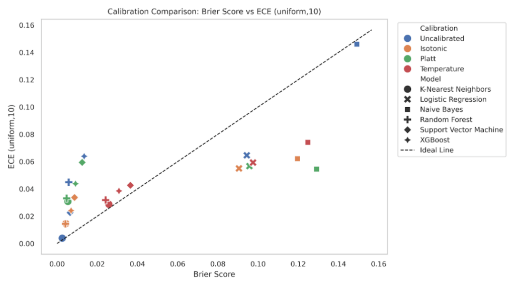
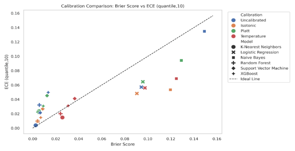
To explore the relationship between calibration and prediction quality, we plotted Expected Calibration Error (ECE) against the Brier Score for all model-calibration combinations (Figure 16-17). Ideally, well-calibrated and accurate models should lie close to the diagonal line, where ECE and Brier Score are proportionally aligned. We plotted ECE (uniform, K = 10) against the Brier score for every model-calibration pair, with a 45° reference line for proportional agreement (Figure 16). Points in the lower left indicate both low Brier and low ECE. XGBoost and Random Forest cluster close to this region under isotonic and Platt, consistent with the grouped bar results that showed small Brier and small ECE after calibration. Logistic Regression sits mid-left, where Brier is modest and ECE varies by method, with isotonic typically lowest. K-Nearest Neighbors and Support Vector Machine show larger spread, and their uncalibrated states lie below the diagonal with small Brier but noticeably higher ECE, matching their reliability curves that showed local miscalibration at low and mid probabilities. Naive Bayes forms the upper-right cloud, reflecting both high Brier and high ECE when uncalibrated, with clear leftward and downward shifts after calibration.

Repeating the plot with quantile binning reduces ECE values across most points while preserving the relative ordering (Figure 17). This mirrors the sensitivity analysis where quantile ECE was systematically lower than uniform ECE. Tree models remain in the lower-left quadrant, Logistic Regression is slightly shuffled & moves closer to the diagonal under isotonic, and KNN continues to show higher ECE than its Brier alone would suggest in the uncalibrated and Platt states. Naive Bayes still separates from the rest, but calibration methods shift it downward and left. The consistency of these patterns across both binning schemes supports the conclusion that models with better Brier also tend to have better calibration, while ECE exposes cases where apparently small Brier can hide meaningful miscalibration.

3.5. Sharpness of predicted probabilities

Sharpness, measured as the variance of predicted probabilities, summarizes how concentrated a model’s probabilities are. Larger variance means more confident predictions; smaller variance means flatter, more conservative outputs.

Across all conditions, KNN is the sharpest. The uncalibrated KNN attains the highest variance at 0.249, and remains high after calibration, 0.240 with isotonic and 0.230 with temperature, with a modest reduction under Platt to 0.223. Tree ensembles are also highly sharp, but their behavior differs by calibration method. Random Forest rises from 0.211 uncalibrated to 0.239 with isotonic, with smaller values for Platt (0.222) and temperature (0.226). XGBoost shows a similar pattern, 0.196 uncalibrated, 0.231 isotonic, 0.214 temperature, 0.212 Platt. These results indicate that isotonic leaves ensemble predictions are confident, while Platt and temperature introduce mild smoothing.

For margin-based and linear models, calibration tends to smooth more. SVM drops from initial 0.232 uncalibrated to 0.223 with isotonic, 0.207 with temperature, and 0.199 with Platt. Logistic Regression falls from 0.157 uncalibrated to 0.164 isotonic, 0.150 temperature, and 0.139 Platt. Naive Bayes exhibits the largest reduction, from 0.229 uncalibrated to 0.166 temperature, 0.134 isotonic, and 0.102 Platt, consistent with its strong decrease in ECE and Log Loss in Table 9.

Isotonic often preserves or slightly increases sharpness for the ensembles while reducing ECE and Log Loss, suggesting better-positioned confidence without blunting predictions. Also, Platt and temperature systematically soften LR, SVM, and NB, which can be desirable when the uncalibrated model is overconfident, as evidenced by their reliability curves in Figure 6-9 and Spiegelhalter’s statistics in Figure 15.

4. Interpretation of Results

This study demonstrates the impact of post-hoc calibration methods on model confidence, calibration quality, and statistical reliability in heart disease prediction. Isotonic regression remained the most effective calibrator for several models, but its advantage was model-dependent. In our cross-validated analysis, Random Forest, XGBoost, Logistic Regression, and Naive Bayes showed consistent improvements under isotonic calibration across Brier, ECE, and Log Loss, while Support Vector Machine and K-Nearest Neighbors were best left uncalibrated on the calibration metrics and likelihood, with temperature scaling often worsening discrimination. These conclusions are supported by the grouped calibration plots with 95% confidence intervals and the permutation tests that compare calibrated to uncalibrated fold by fold (Tables 8-10, Figures 11-15). As an illustration, Random Forest’s ECE and Log Loss decrease substantially under isotonic relative to uncalibrated in the grouped plots, and Naive Bayes exhibits the largest drops among all models. These effects are mirrored by near-zero Spiegelhalter Z with higher p after calibration in several models, which indicates no detectable miscalibration at fold scale while recognizing that non-significant p does not prove perfect calibration [61].

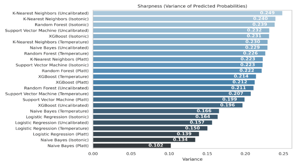
These findings support the theory that sigmoid calibration is most suitable when miscalibration is close to a logistic shift, whereas isotonic regression can correct more complex, monotone distortions [7], [9]. Temperature scaling provides a single-parameter softness control, but it shifts Accuracy and F1 across all models and frequently increased Log Loss, so it should be applied with caution here [5]. The comparative nature of our analysis is crucial. We based inferences on cross-validated fold means with confidence intervals, and on paired permutation tests that quantify whether calibrated metrics are better than uncalibrated under the matched fold design, directly addressing requests for statistical comparison rather than isolated point estimates.

In clinical applications, where predicted risks inform communication and thresholds, miscalibrated models can convey inappropriate levels of confidence, complicating risk discussions and the consistency of threshold-based decisions without necessarily improving patient-level utility. For example, Naive Bayes before calibration produced extreme probabilities with poor alignment to outcomes, which post-calibration corrected, lowering Brier and Log Loss and improving Z and p toward values consistent with good calibration. This highlights the need for calibration pipelines in AI-assisted diagnostics to improve trustworthiness and reduce the risk that probability outputs misrepresent uncertainty [72]. Reliability diagrams built from out-of-fold predictions with Wilson intervals and per-bin counts further illustrate these corrections while avoiding test-set leakage [5][56]. Together with the sharpness analysis, this shows when confidence is well in line with observed risk and when it is not.

A key methodological contribution is the joint use of multiple calibration summaries, guidance on clinical presentation of calibration and reporting practices supports this multi-metric approach [52]. Previous work often reported only one metric such as Brier or ECE [5], [73]. We combined Brier, ECE, Log Loss, Spiegelhalter’s Z, p-value, and Sharpness across six classifiers, and we visualized their relationships with grouped plots and Brier versus ECE scatterplots. The scatterplots show that points move down and left after isotonic for the tree ensembles and Naive Bayes, indicating lower calibration error and lower probabilistic loss, while SVM and KNN tend to cluster closer to their uncalibrated states, consistent with their preference to remain uncalibrated. The ECE sensitivity analysis confirms that equal-frequency binning yields smaller ECE than equal-width on average, with a positive median difference and a paired test p below conventional threshold. We therefore report both ECE variants, interpret their magnitudes cautiously, and base primary claims on the convergence of multiple metrics rather than a single summary [5], [56].

Another contribution of this work is a reproducible evaluation framework for post-hoc calibration in binary heart disease prediction that couples strict leakage control with fold-conscious uncertainty and paired comparative testing. Some models, notably Naive Bayes and Random Forest, benefit substantially from isotonic calibration, while others, such as KNN and SVM, do not. By introducing sharpness alongside calibration, we examine correctness and the confidence dispersion, which is essential for risk stratification and model auditability [74]. Throughout, all preprocessing, threshold selection by Youden’s J inside an inner loop, and calibration were fit on training data only, never on the test set, which reduces optimistic bias and supports statistically valid inference [44], [75], [76].

From an operational standpoint, the calibration procedures used here are lightweight and feasible to maintain. Platt and temperature scaling add negligible compute at inference and only a small fit cost on held-out training predictions, while isotonic regression remains inexpensive at structured clinical feature data. For integration, the same nested cross-validated approach can be embedded in routine retraining to provide continuous calibration as data drift is detected, for example by monitoring ECE and Log Loss on recent cases and triggering recalibration when control limits are exceeded. Because probability calibration can change subgroup error profiles, fairness should be checked pre and post-calibration, for instance by reporting calibration curves, ECE, and Brier stratified by demographic groups, and by tracking stability under distribution shift. In our setting, the per-model recommendations are actionable, isotonic for tree ensembles and Naive Bayes, uncalibrated for SVM and KNN, and cautious use of temperature scaling. This preserves inference speed and aligns with a periodic recalibration policy that is straightforward to implement in clinical pipelines.

This study is limited by the size of the dataset (N=1,025), which can increase variability in binned metrics and in Z, even with Wilson intervals and cross-validated designs. We did not include an external cohort, so generalizability remains to be confirmed on independent populations. We focused on Platt, Isotonic, and Temperature, leaving alternatives such as beta calibration or Bayesian binning to future work. We also did not include decision-curve analysis in the main results, which would connect calibrated probabilities to clinical net benefit and we did not integrate model interpretability or explainability analysis. Future research should extend the framework to external and temporal validation, add decision-curve analysis under fixed thresholds selected by Youden’s J, evaluate alternative calibrators, and incorporate explainability to link calibrated risk with feature attributions in support of clinical review.

5. Conclusion

This study evaluated the calibration performance of six classification models for heart disease prediction using post-hoc techniques and multiple uncertainty metrics. While several models achieved strong discrimination, their probability estimates were not always aligned with observed outcomes. This confirms the need to assess probability quality in addition to accuracy and AUC ROC.

Across methods and models, post-hoc calibration improved probability alignment in a model-dependent way. Isotonic regression yielded the most consistent gains in Brier score, ECE, and Log Loss for Random Forest, XGBoost, Logistic Regression, and Naive Bayes, with effects verified under cross-validated estimation, bootstrap intervals, and paired permutation tests. Spiegelhalter’s Z and p provided complementary evidence for absolute calibration, interpreted cautiously given sample size. In contrast, Support Vector Machine and K-Nearest Neighbors were best left uncalibrated on these metrics. Temperature scaling was included for completeness, but in this setting, it often increased Log Loss and affected discrimination.

The study contributes a reproducible calibration-evaluation framework for structured clinical predictors. Preprocessing, threshold selection via Youden’s J, and all calibrators were fit on training data within cross-validation, then applied to matched validation folds and only finally to the held-out test set. Reliability diagrams were built from out-of-fold predictions with Wilson intervals and bin counts. ECE was reported in two variants, equal-width and equal-frequency, and a paired sensitivity analysis showed lower values under quantile binning without changing the qualitative ranking. Sharpness was reported alongside calibration to characterize confidence concentration, helping to interpret when improvements reflect better aligned probabilities rather than simple smoothing.

These results indicate that isotonic calibration is a strong default for tree ensembles and Naive Bayes under this workflow, that Logistic Regression benefits from Isotonic, and that SVM and KNN may not require calibration. The framework balances calibration and discrimination by using a single threshold per model chosen with Youden’s J inside the training folds, which mirrors a stable operating policy. The overall recommendation is to evaluate calibration routinely with fold-aware uncertainty, to select the calibration method by empirical evidence on the target data, and to deploy periodic recalibration with monitoring for drift.

Conflict of Interest

The authors declare that no funding was received from any affiliated institution for this research. The work was conducted independently and the views expressed are solely those of the authors.

Acknowledgement

We would like to acknowledge Emmanuel Ughoo (Independent Researcher, Southampton, UK) for his contributions to the conceptualization of this work, including early-stage brainstorming and shaping the initial study direction.

Data and Code Availability

The dataset and code supporting the findings of this study is available from the corresponding author on reasonable request.

1. World Health Organization, “Cardiovascular diseases (CVDs),” World Health Organization, Jul. 2025.
2. D. Dey, P. J. Slomka, P. Leeson, D. Comaniciu, M. L. Bots, “Artificial intelligence in cardiovascular imaging: JACC state-of-the-art review,” Journal of the American College of Cardiology, vol. 73, no. 11, pp. 1317–1335, 2019, doi: 10.1016/j.jacc.2018.12.054.
3. S. Srinivasan, S. Gunasekaran, S. K. Mathivanan, “An active learning machine technique-based prediction of cardiovascular heart disease from UCI-repository database,” Scientific Reports, vol. 13, art. no. 13588, 2023, doi: 10.1038/s41598-023-40717-1.
4. S. F. Weng, J. Reps, J. Kai, J. M. Garibaldi, N. Qureshi, “Can machine-learning improve cardiovascular risk prediction using routine clinical data?,” PLOS ONE, vol. 12, no. 4, art. no. e0174944, 2017, doi: 10.1371/journal.pone.0174944.
5. C. Guo, G. Pleiss, Y. Sun, K. Q. Weinberger, “On calibration of modern neural networks,” in Proc. 34th Int. Conf. Machine Learning (ICML), 2017, pp. 1321–1330, doi: 10.48550/arXiv.1706.04599.
6. H. Jiang, B. Kim, M. Y. Guan, M. Gupta, “To trust or not to trust a classifier,” in Proc. 32nd Int. Conf. Neural Information Processing Systems (NeurIPS), Montreal, Canada, 2018, pp. 5546–5557.
7. B. Zadrozny, C. Elkan, “Transforming classifier scores into accurate multiclass probability estimates,” in Proc. 8th ACM SIGKDD Int. Conf. Knowledge Discovery and Data Mining, 2002, pp. 694–699, doi: 10.1145/775047.775151.
8. S. Tonekaboni, S. Joshi, M. D. McCradden, A. Goldenberg, “What clinicians want: contextualizing explainable machine learning for clinical end use,” in Proc. 4th Machine Learning for Healthcare Conf. (PMLR, vol. 106), 2019, pp. 359–380. [Online]. Available: https://proceedings.mlr.press/v106/tonekaboni19a.html
9. A. Niculescu-Mizil, R. Caruana, “Predicting good probabilities with supervised learning,” in Proc. 22nd Int. Conf. Machine Learning (ICML), 2005, pp. 625–632, doi: 10.1145/1102351.1102430.
10. M. M. Ali, B. K. Paul, K. Ahmed, F. M. Bui, J. M. W. Quinn, and M. A. Moni, “Heart disease prediction using supervised machine learning algorithms: Performance analysis and comparison,” Computers in Biology and Medicine, vol. 136, art. no. 104672, 2021, doi: 10.1016/j.compbiomed.2021.104672.
11. S. Ghosh, M. A. Islam, “Performance evaluation and comparison of heart disease prediction using machine learning methods with elastic net feature selection,” American Journal of Applied Mathematics and Statistics, vol. 11, no. 2, pp. 35–49, 2023, doi: 10.12691/ajams-11-2-1.
12. G. N. Ahmad, Shafiullah, H. Fatima, M. Abbas, O. Rahman, Imdadullah, M. S. Alqahtani, “Mixed machine learning approach for efficient prediction of human heart disease by identifying the numerical and categorical features,” Applied Sciences, vol. 12, no. 15, art. no. 7449, 2022, doi: 10.3390/app12157449.
13. M. Sayadi, V. Varadarajan, F. Sadoughi, S. Chopannejad, M. Langarizadeh, “A machine learning model for detection of coronary artery disease using noninvasive clinical parameters,” Life, vol. 12, no. 11, art. no. 1933, 2022, doi: 10.3390/life12111933.
14. L. Deng, K. Lu, H. Hu, “An interpretable LightGBM model for predicting coronary heart disease: Enhancing clinical decision-making with machine learning,” PLOS ONE, vol. 20, no. 9, art. no. e0330377, 2025, doi: 10.1371/journal.pone.0330377.
15. H. El-Sofany, B. Bouallegue, Y. M. A. El-Latif, “A proposed technique for predicting heart disease using machine learning algorithms and an explainable AI method,” Scientific Reports, vol. 14, art. no. 23277, 2024, doi: 10.1038/s41598-024-74656-2.
16. A. -D. Samaras, S. Moustakidis, I. D. Apostolopoulos, N. Papandrianos, E. Papageorgiou, “Classification models for assessing coronary artery disease instances using clinical and biometric data: an explainable man-in-the-loop approach,” Scientific Reports, vol. 13, art. no. 6668, 2023, doi: 10.1038/s41598-023-33500-9.
17. T. Vu et al., “Machine learning model for predicting coronary heart disease risk: Development and validation using insights from a Japanese population-based study,” JMIR Cardio, vol. 9, art. no. e68066, 2025, doi: 10.2196/68066.
18. M. U. Rehman, S. Naseem, A. U. R. Butt, “Predicting coronary heart disease with advanced machine learning classifiers for improved cardiovascular risk assessment,” Scientific Reports, vol. 15, art. no. 13361, 2025, doi: 10.1038/s41598-025-96437-1.
19. G. M. Rao, D. Ramesh, V. Sharma, “AttGRU-HMSI: Enhancing heart disease diagnosis using hybrid deep learning approach,” Scientific Reports, vol. 14, art. no. 7833, 2024, doi: 10.1038/s41598-024-56931-4.
20. J. You, Y. Guo, J. J. Kang, “Development of machine learning-based models to predict 10-year risk of cardiovascular disease: A prospective cohort study,” Stroke and Vascular Neurology, vol. 8, no. 6, pp. 475–485, 2023, doi: 10.1136/svn-2023-002332.
21. C. Li et al., “Improving cardiovascular risk prediction through machine learning modelling of irregularly repeated electronic health records,” European Heart Journal – Digital Health, vol. 5, no. 1, pp. 30–40, 2024, doi: 10.1093/ehjdh/ztad058.
22. J. W. Hughes, J. Tooley, J. T. Soto, “A deep learning-based electrocardiogram risk score for long term cardiovascular death and disease,” npj Digit. Med., vol. 6, art. no. 169, 2023, doi: 10.1038/s41746-023-00916-6.
23. Y. Xi, H. Wang, N. Sun, “Machine learning outperforms traditional logistic regression and offers new possibilities for cardiovascular risk prediction: A study involving 143,043 Chinese patients with hypertension,” Frontiers in Cardiovascular Medicine, vol. 9, art. no. 1025705, 2022, doi: 10.3389/fcvm.2022.1025705.
24. S. Y. Cho, S. H. Kim, S. H. Kang, “Pre-existing and machine learning-based models for cardiovascular risk prediction,” Scientific Reports, vol. 11, art. no. 8886, 2021, doi: 10.1038/s41598-021-88257-w.
25. R. Khera, J. Haimovich, N. C. Hurley et al., “Use of machine learning models to predict death after acute myocardial infarction,” JAMA Cardiology, vol. 6, no. 6, pp. 633–641, 2021, doi: 10.1001/jamacardio.2021.0122.
26. L. R. Guarneros-Nolasco, N. A. Cruz-Ramos, G. Alor-Hernández, L. Rodríguez-Mazahua, J. L. Sánchez-Cervantes, “Identifying the main risk factors for cardiovascular diseases prediction using machine learning algorithms,” Mathematics, vol. 9, no. 20, art. no. 2537, 2021, doi: 10.3390/math9202537.
27. L. Yang, H. Wu, X. Jin, “Study of cardiovascular disease prediction model based on random forest in eastern China,” Scientific Reports, vol. 10, art. no. 5245, 2020, doi: 10.1038/s41598-020-62133-5.
28. A. M. Alaa, T. Bolton, E. Di Angelantonio, J. H. F. Rudd, M. van der Schaar, “Cardiovascular disease risk prediction using automated machine learning: A prospective study of 423,604 UK Biobank participants,” PLOS ONE, vol. 14, no. 5, art. no. e0213653, 2019, doi: 10.1371/journal.pone.0213653.
29. S. F. Weng, J. Reps, J. Kai, J. M. Garibaldi, N. Qureshi, “Can machine-learning improve cardiovascular risk prediction using routine clinical data?,” PLOS ONE, vol. 12, no. 4, art. no. e0174944, 2017, doi: 10.1371/journal.pone.0174944.
30. P. J. Rousseeuw, C. Croux, “Alternatives to the median absolute deviation,” Journal of the American Statistical Association, vol. 88, no. 424, pp. 1273–1283, Dec. 1993, doi: 10.1080/01621459.1993.10476408.
31. C. Y. J. Peng, K. L. Lee, G. M. Ingersoll, “An introduction to logistic regression analysis and reporting,” Journal of Educational Research, vol. 96, no. 1, pp. 3–14, 2002, doi: 10.1080/00220670209598786.
32. T. S. Furey et al., “Support vector machine classification and validation of cancer tissue samples using microarray expression data,” Bioinformatics, vol. 16, no. 10, pp. 906–914, 2000, doi: 10.1093/bioinformatics/16.10.906.
33. L. Breiman, “Random forests,” Machine Learning, vol. 45, no. 1, pp. 5–32, Oct. 2001, doi: 10.1023/A:1010933404324.
34. T. Chen, C. Guestrin, “XGBoost: A scalable tree boosting system,” in Proc. 22nd ACM SIGKDD Int. Conf. Knowledge Discovery and Data Mining (KDD), 2016, pp. 785–794, doi: 10.1145/2939672.2939785.
35. T. Cover, P. Hart, “Nearest neighbor pattern classification,” IEEE Transactions on Information Theory, vol. 13, no. 1, pp. 21–27, 1967, doi: 10.1109/TIT.1967.1053964.
36. G. H. John, P. Langley, “Estimating continuous distributions in Bayesian classifiers,” in Proc. 11th Conf. Uncertainty in Artificial Intelligence (UAI ’95), Montreal, QC, Canada, 1995, pp. 338–345, doi: 10.5555/2074158.2074196.
37. M. Feurer, F. Hutter, “Hyperparameter optimization,” in Automated Machine Learning: Methods, Systems, Challenges, F. Hutter, L. Kotthoff, and J. Vanschoren, Eds. Cham, Switzerland: Springer, 2019, pp. 3–33, doi: 10.1007/978-3-030-05318-5_1.
38. W. Nugraha, A. Sasongko, “Hyperparameter tuning on classification algorithm with grid search,” Sistemasi: Jurnal Sistem Informasi, vol. 11, no. 2, pp. 391–401, 2022, doi: 10.32520/stmsi.v11i2.1750.
39. G. N. Ahmad, H. Fatima, S. Ullah, A. S. Saidi, “Efficient medical diagnosis of human heart diseases using machine learning techniques with and without GridSearchCV,” IEEE Access, vol. 10, pp. 80151–80173, 2022, doi: 10.1109/ACCESS.2022.3165792.
40. A. Ogunpola, F. Saeed, S. Basurra, A. Albarrak, S. Qasem, “Machine learning-based predictive models for detection of cardiovascular diseases,” Diagnostics, vol. 14, no. 2, art. no. 144, 2024, doi: 10.3390/diagnostics14020144.
41. Z. S. Dunias, B. Van Calster, D. Timmerman, A.-L. Boulesteix, M. Van Smeden, “A comparison of hyperparameter tuning procedures for clinical prediction models: A simulation study,” Statistics in Medicine, vol. 43, no. 6, pp. 1119–1134, 2024, doi: 10.1002/sim.9932.
42. W. J. Youden, “Index for rating diagnostic tests,” Cancer, vol. 3, no. 1, pp. 32–35, 1950, doi: 10.1002/1097-0142(1950).
43. R. Fluss, D. Faraggi, B. Reiser, “Estimation of the Youden Index and its associated cutoff point,” Biometrical Journal, vol. 47, no. 4, pp. 458–472, 2005, doi: 10.1002/bimj.200410135.
44. S. Varma, R. Simon, “Bias in error estimation when using cross-validation for model selection,” BMC Bioinformatics, vol. 7, art. no. 91, 2006, doi: 10.1186/1471-2105-7-91.
45. C. Nadeau, Y. Bengio, “Inference for the generalization error,” Machine Learning, vol. 52, pp. 239–281, 2003, doi: 10.1023/A:1024068626366.
46. T. SaitoM. Rehmsmeier, “The precision-recall plot is more informative , han the ROC plot when evaluating binary classifiers on imbalanced datasets,” PLOS ONE, vol. 10, no. 3, art. no. e0118432, 2015, doi: 10.1371/journal.pone.0118432.
47. T. Fawcett, “An introduction to ROC analysis,” Pattern Recognition Letters, vol. 27, no. 8, pp. 861–874, 2006, doi: 10.1016/j.patrec.2005.10.010.
48.  J. Davis, M. Goadrich, “The relationship between precision-recall and ROC curves,” in Proc. 23rd Int. Conf. Machine Learning (ICML), 2006, pp. 233–240, doi: 10.1145/1143844.1143874.
49. E. W. Steyerberg, Clinical Prediction Models: A Practical Approach to Development, Validation, and Updating, 2nd ed. Springer, 2019, doi: 10.1007/978-3-030-16399-0.
50. D. Chicco, G. Jurman, “The advantages of the Matthews correlation coefficient (MCC) over F1 score and accuracy in binary classification evaluation,” BMC Genomics, vol. 21, art. no. 6, 2020, doi: 10.1186/s12864-019-6413-7.
51. C. Penso, L. Frenkel, J. Goldberger, “Confidence calibration of a medical imaging classification system that is robust to label noise,” IEEE Transactions on Medical Imaging, vol. 43, no. 6, pp. 2050–2060, 2024, doi: 10.1109/TMI.2024.3353762.
52. B. Van Calster, D. J. McLernon, M. van Smeden, “Calibration: The Achilles heel of predictive analytics,” BMC Medicine, vol. 17, art. no. 230, 2019, doi: 10.1186/s12916-019-1466-7.
53. M. Kull, T. D. Filho, P. A. Flach, “Beyond sigmoids: How to obtain well-calibrated probabilities from binary classifiers with beta calibration,” Electronic Journal of Statistics, vol. 11, pp. 5052–5080, 2017, doi: 10.1214/17-EJS1338SI.
54. R. E. Barlow, H. D. Brunk, “The isotonic regression problem and its dual,” Journal of the American Statistical Association, vol. 67, no. 337, pp. 140–147, Mar. 1972, doi: 10.1080/01621459.1972.10481216.
55. T. Gneiting, F. Balabdaoui, A. E. Raftery, “Probabilistic forecasts, calibration and sharpness,” Journal of the Royal Statistical Society: Series B (Statistical Methodology), vol. 69, no. 2, pp. 243–268, Apr. 2007, doi: 10.1111/j.1467-9868.2007.00587.x.
56. G. Bröcker, L. A. Smith, “Increasing the reliability of reliability diagrams,” Weather and Forecasting, vol. 22, no. 3, pp. 651–661, 2007, doi: 10.1175/WAF993.1.
57. M. Assel, D. Sjoberg, A. Vickers, “The Brier score does not evaluate the clinical utility of diagnostic tests or prediction models,” Diagnostic and Prognostic Research, vol. 1, 2017, doi: 10.1186/s41512-017-0020-3.
58. D. R. Cox, “The regression analysis of binary sequences,” Journal of the Royal Statistical Society: Series B (Methodological), vol. 20, no. 2, pp. 215–242, 1958, doi: 10.1111/j.2517-6161.1958.tb00292.x.
59. B. Efron, R. J. Tibshirani, An Introduction to the Bootstrap, 1st ed. Chapman and Hall/CRC, 1994, doi: 10.1201/9780429246593.
60. L. D. Brown, T. T. Cai, A. DasGupta, “Interval estimation for a binomial proportion,” Statistical Science, vol. 16, no. 2, pp. 101–133, 2001, doi: 10.1214/ss/1009213286.
61. D. J. Spiegelhalter, “Probabilistic prediction in patient management and clinical trials,” Statistics in Medicine, vol. 5, no. 5, pp. 421–433, Sep. 1986, doi: 10.1002/sim.4780050506.
62. R. A. Fisher, The Design of Experiments. Oliver & Boyd, 1935.
63. P. Good, Permutation, Parametric, and Bootstrap Tests of Hypotheses, 3rd ed. Springer, 2005, doi: 10.1007/b138696.
64. F. Wilcoxon, “Individual comparisons by ranking methods,” Biometrics Bulletin, vol. 1, no. 6, pp. 80–83, 1945, doi: 10.2307/3001968.
65. O. Rainio, J. Teuho, R. Klén, “Evaluation metrics and statistical tests for machine learning,” Scientific Reports, vol. 14, art. no. 6086, 2024, doi: 10.1038/s41598-024-56706-x.
66. E. F. Schisterman, N. J. Perkins, A. Liu, H. Bondell, “Optimal cut-point and its corresponding Youden Index to discriminate individuals using pooled blood samples,” Epidemiology, vol. 16, no. 1, pp. 73–81, 2005, doi: 10.1097/01.ede.0000147512.81966.ba.
67. O. Rainio, J. Tamminen, M. S. Venäläinen, “Comparison of thresholds for a convolutional neural network classifying medical images,” International Journal of Data Science and Analytics, vol. 20, pp. 2093–2099, 2025, doi: 10.1007/s41060-024-00584-z.
68. H.-T. Lin, C.-J. Lin, R. C. Weng, “A note on Platt’s probabilistic outputs for support vector machines,” Machine Learning, vol. 68, pp. 267–276, 2007, doi: 10.1007/s10994-007-5018-6.
69. B. Böken, “On the appropriateness of Platt scaling in classifier calibration,” Information Systems, vol. 95, art. no. 101641, 2021, doi: 10.1016/j.is.2020.101641.
70. M. P. Naeini, G. F. Cooper, M. Hauskrecht, “Obtaining well calibrated probabilities using Bayesian binning,” in Proc. 29th AAAI Conf. Artificial Intelligence (AAAI), Austin, TX, USA, 2015, pp. 2901–2907, doi: 10.1609/aaai.v29i1.9602.
71. Y. Huang, W. Li, F. Macheret, R. A. Gabriel, L. Ohno-Machado, “A tutorial on calibration measurements and calibration models for clinical prediction models,” Journal of the American Medical Informatics Association, vol. 27, no. 4, pp. 621–633, Apr. 2020, doi: 10.1093/jamia/ocz228.
72. E. W. Steyerberg et al., “Assessing the performance of prediction models: A framework for traditional and novel measures,” Epidemiology, vol. 21, no. 1, pp. 128–138, 2010, doi: 10.1097/EDE.0b013e3181c30fb2.
73. X. Jiang, M. Osl, J. Kim, L. Ohno-Machado, “Calibrating predictive model estimates to support personalized medicine,” Journal of the American Medical Informatics Association, vol. 19, no. 2, pp. 263–274, 2012, doi: 10.1136/amiajnl-2011-000291.
74. V. Kuleshov, N. Fenner, S. Ermon, “Accurate uncertainties for deep learning using calibrated regression,” in Proc. 35th Int. Conf. Machine Learning (ICML), 2018, pp. 2796–2804, doi: 10.48550/arXiv.1807.00263.
75. D. Krstajic, L. J. Buturovic, D. E. Leahy, “Cross-validation pitfalls when selecting and assessing regression and classification models,” Journal of Cheminformatics, vol. 6, art. no. 10, 2014, doi: 10.1186/1758-2946-6-10.
76. G. C. Cawley, N. L. C. Talbot, “On over-fitting in model selection and subsequent selection bias in performance evaluation,” Journal of Machine Learning Research, vol. 11, pp. 2079–2107, 2010.

Citations by Dimensions

Citations by PlumX

Crossref Citations

1. Peter Adebayo Odesola, Adewale Alex Adegoke, Idris Babalola, “Comparative Analysis of Supervised Machine Learning Models for PCOS Prediction Using Clinical Data”, Journal of Engineering Research and Sciences, vol. 4, no. 6, pp. 16–26, 2025. doi: 10.55708/js0406003
2. Peter Adebayo Odesola, Adewale Alex Adegoke, Idris Babalola, “Fire Type Classification in the USA Using Supervised Machine Learning Techniques”, Journal of Engineering Research and Sciences, vol. 4, no. 6, pp. 1–8, 2025. doi: 10.55708/js0406001
3. Peter Adebayo Odesola, Adewale Alex Adegoke, Idris Babalola, “AI-Driven Digital Transformation: Challenges and Opportunities”, Journal of Engineering Research and Sciences, vol. 4, no. 4, pp. 8–19, 2025. doi: 10.55708/js0404002
4. Peter Adebayo Odesola, Adewale Alex Adegoke, Idris Babalola, “Enhancing Python Code Embeddings: Fusion of Code2vec with Large Language Models”, Journal of Engineering Research and Sciences, vol. 4, no. 1, pp. 1–7, 2025. doi: 10.55708/js0401001
5. Peter Adebayo Odesola, Adewale Alex Adegoke, Idris Babalola, “Enhancing Mental Health Support in Engineering Education with Machine Learning and Eye-Tracking”, Journal of Engineering Research and Sciences, vol. 3, no. 10, pp. 69–75, 2024. doi: 10.55708/js0310007