Explainable AI for SSD Failure Prediction: Using LIME and SHAP for Transparency

(This article belongs to the Section Artificial Intelligence – Computer Science (AIC))
Export Citations
Cite
Kumar, S. K. (2026). Explainable AI for SSD Failure Prediction: Using LIME and SHAP for Transparency. Journal of Engineering Research and Sciences, 5(4), 1–16. https://doi.org/10.55708/js0504001
Saurav Kant Kumar. "Explainable AI for SSD Failure Prediction: Using LIME and SHAP for Transparency." Journal of Engineering Research and Sciences 5, no. 4 (April 2026): 1–16. https://doi.org/10.55708/js0504001
S.K. Kumar, "Explainable AI for SSD Failure Prediction: Using LIME and SHAP for Transparency," Journal of Engineering Research and Sciences, vol. 5, no. 4, pp. 1–16, Apr. 2026, doi: 10.55708/js0504001.
Artificial Intelligence (AI) has become increasingly crucial for modern data centers for automating tasks ranging from anomaly detection to predictive maintenance. Nevertheless, a significant limitation of underlying machine learning (ML) models is their “black box” nature. This lack of transparency limits trust among stakeholders who require visibility into model decisions. We address this lack of transparency by evaluating explainable AI techniques within an SSD failure prediction pipeline to improve interpretability and operational trust. Our study makes the following three main contributions. First, we provide a large-scale empirical evaluation of explainable AI techniques (LIME and SHAP) within an SSD failure prediction pipeline under realistic temporal validation and deployment constraints. Second, we provide a qualitative comparison of LIME and SHAP, focusing on their roles in local and global interpretability and their practical behavior in SSD failure prediction. Third, we analyze model performance from an operational perspective using a cost-sensitive framework, demonstrating how explainability supports decision-making in data center environments. To address temporal data leakage and model robustness, we evaluate our approach on a temporal split with 10,637,778 training records and 5,499,337 test records from the Alibaba dataset, which contains data from over 500,000 SSDs. The tuned XGBoost model achieved a recall of 67.98%, precision of 4.43%, and false alarm rate of 0.1878, by optimizing a custom "Safety-First" cost function at a decision threshold of 0.680, effectively functioning as a high-sensitivity screening tool. This approach resulted in an estimated net operational savings of $13.42 million compared to baseline maintenance strategies. Additionally, the findings show that LIME generates intuitive, human-readable justifications for individual predictions and SHAP explains the model at both global and local levels. Integration of an explainable AI layer to ML pipelines turns “black box” models into systems that are easy to understand and verify, which makes them more trustworthy and reliable.
1. Introduction
Global data volume has grown rapidly in recent years because far more individuals have access to the internet, more people are using cloud computing, and the use of digital devices has exploded. With IDC projecting global data volumes to reach 175 zettabytes (ZB) by 2025, data centers are deploying massive SSD fleets that continuously generate telemetry data, including SMART metrics, wear indicators, latency measurements, and temperature readings [1], [2]. At the same time, the amount of computing power needed for modern AI models has doubled every few months in the past [3]. Because of this, data center technicians must work hard to keep their systems running 100% of the time to make sure they are reliable and don’t cause service outages. This necessitates predictive maintenance, anomaly detection, accurate SSD failure prediction, and the use of explainable AI to validate the results [18].
To predict an SSD failure, it’s necessary to train complex machine learning (ML) models on telemetry data. However, these models are “black boxes”, which means it’s hard to know how they make predictions [2], [4], [5]. Although these models can be highly accurate, their internal decision-making process is often opaque to users, operations managers, reliability engineers, and compliance teams who must trust and validate the decisions generated by these models [6], [7]. When a model predicts that a specific SSD has a high probability of failure, stakeholders must be able to understand the reasoning behind that prediction. This lack of transparency makes it difficult to verify predictions, ensure accountability, and build confidence in the system [8], [9]. Consequently, there is a need for explainable AI techniques to make SSD failure prediction more interpretable, transparent, and operationally trustworthy [10], [11].
The importance of explainable AI is not limited to operational trust in the model predictions; it is becoming a statutory requirement [6], [8], [12]. Many countries have introduced strong data protection and AI governance frameworks, including the GDPR and AI Act of the EU, CCPA and NIST AI Risk Management Framework in the United States, and global regulations such as PIPEDA (Canada), LGPD (Brazil), POPIA (South Africa), and China’s PIPL [8], [9], [13], [15]. These laws call for transparency, traceability, and accountability in automated systems, thus augmenting the significance of explainable AI methodologies [6], [14]. In the United States, agencies such as the National Institute of Standards and Technology (NIST), the Federal Trade Commission (FTC), and the Cybersecurity and Infrastructure Security Agency (CISA) are developing guidelines for the trustworthy deployment of AI in critical infrastructure, where model interpretability is essential for ensuring safety, auditability, and regulatory compliance [15], [16], [17]. Insufficient or confusing explanations for how a machine-learning model reaches a failure prediction can result in compliance violations, loss of customer and stakeholder trust, and difficulties meeting industry requirements for safety, reliability, and fairness in automated decision-making [8], [9].
Advanced machine learning models used for SSD failure prediction, including ensemble approaches such as Random Forest, XGBoost, and LightGBM, demonstrate strong predictive performance; however, they often lack interpretability [2], [10], [20]. Stakeholders prefer not only accurate predictions of failures that are about to happen, but also detailed explanations of how these predictions are made [7], [11]. From an operational standpoint, stakeholders need to pinpoint exactly which SMART attributes are triggering a failure alert, while also understanding how the model adapts to different SSD vendors and changing workloads [18], [20].
Although LIME and SHAP are widely used post-hoc explanation techniques, there remains limited empirical evidence regarding their effectiveness in large-scale SSD failure prediction systems evaluated under realistic temporal validation constraints. Also, these models must be validated against temporal data leakage to ensure that historical patterns effectively generalize to future failure events.
This paper focuses on the interpretability and operational viability of machine learning models for SSD failure prediction and makes the following contributions:
- We train and evaluate the performance of Random Forest, XGBoost, and LightGBM using a strict temporal walk-forward split of 16,137,115 telemetry records (10,637,778 training and 5,499,337 test records) spanning 90,761 unique SSDs from the Alibaba dataset.This scale and validation strategy ensure real-world predictive integrity by eliminating the temporal data leakage often introduced by random train–test splits in failure prediction studies.
- We systematically evaluate LIME and SHAP as diagnostic tools for SSD failure prediction, testing their ability to provide interpretable explanations that support auditing, transparency, and regulatory requirements such as the “Right to Explanation” under frameworks including GDPR and the NIST AI Risk Management Framework.
- We apply a cost-sensitive decision framework that integrates threshold optimization with an operational cost model, enabling economically efficient failure prediction under asymmetric risk conditions.
- We evaluate the integration of explainable AI techniques within an SSD failure prediction pipeline to improve interpretability and support operational decision-making.
This paper is structured as follows: Section 2 reviews related work on regulatory frameworks, explainable AI, and SSD failure prediction. Section 3 describes the methodology and proposed system architecture. In Section 4, we show the experimental results, highlighting how effectively the model worked, an assessment of operational costs, and thorough explainability assessments. Section 5 discusses the strategic implications for data center operators, the economic trade-offs of the “Safety-First” approach, and current limitations. Finally, Section 6 concludes the paper.
2. Related Work
Our research takes inspiration from three domains: regulatory frameworks mandating transparency and explainability, advancements in explainable AI methodologies, and the application of machine learning techniques to predict SSD failures.
2.1. Regulatory Frameworks
The rapid advancement and widespread use of AI, together with the focus on transparency and accountability, have led to the development of regulations and standards on how to use AI [6], [8], [9]. The General Data Protection Regulation (GDPR) and the forthcoming AI Act of the European Union mandate a right to explanation and classify high-risk AI systems, such as those used in critical infrastructure, under strict transparency, documentation, and human-oversight requirements [12], [13]. Similarly, U.S.-based agencies such as NIST, the FTC, and CISA have introduced the AI Risk Management Framework and related guidance to promote trustworthy, auditable AI deployment in enterprise environments [15], [16], [17]. These regulatory initiatives highlight the growing need for explainable AI techniques that enable stakeholders to interpret model predictions, support auditing processes, and ensure responsible deployment of machine learning systems in operational environments. These frameworks illustrate how the focus is shifting from how efficiently the models work to how easy they are to understand, evaluate, and be fair in automated decision-making [6].
2.2. Explainable AI Techniques
While ML and DL models for SSD failure prediction have matured and are able to achieve state-of-the-art performance [2], [20], the field of explainable AI (XAI) has increasingly focused on making these models more interpretable and understandable to stakeholders [10], [11]. XAI methods are generally categorized into intrinsically interpretable models, like linear models and decision trees, and post-hoc explanation techniques that aim to interpret complex black-box models after training. There are several post-hoc XAI methods but LIME (Local Interpretable Model-Agnostic Explanations) and SHAP (SHapley Additive exPlanations) are the most widely adopted methods for understanding model behaviour [4], [5].
LIME explains individual predictions by locally approximating the complex model with an interpretable surrogate model, often a simple linear model or decision tree, around the instance of interest [4]. In SSD failure prediction, LIME highlights which SMART attributes most influenced a specific drive’s failure score, providing transparency at the instance level. Since LIME uses local perturbations of input data, the stability of resulting explanations can vary based on the sampling distribution used to build the local surrogate model.
SHAP uses Shapley values from cooperative game theory to assign each feature an importance score based on all the combinations of features [5]. SHAP provides both local and global interpretability, which lets engineers find the most important elements that affect model predictions across the SSD fleet. SHAP provides more theoretically consistent feature attribution than LIME but is computationally expensive when applied to large datasets or complex ensemble models. Together, LIME and SHAP transform black-box SSD failure models into transparent, auditable systems that reliability teams can trust and validate.
Jakubowski et al. assess LIME and SHAP in the context of asset-failure prediction, differentiating between local and global explanation types and emphasizing the trade-offs between interpretability and model fidelity [10]. Amato et al. evaluate multiple XAI techniques, including LIME and SHAP, in the context of hard disk drive (HDD) health prediction and report that SHAP yields more stable and comprehensive explanations [11]. Lin et al. developed a unified XAI framework that focuses on reliability, transparency, and making industrial systems easy for people to understand [7]. Additional XAI techniques include Integrated Gradients which is a gradient-based attribution technique, along with global interpretation methods such as permutation feature importance and partial dependence analysis. Nonetheless, the systematic and operational-scale adoption of these explanatory techniques for predicting SSD failures in extensive data center environments is still limited, particularly under realistic temporal validation settings and large-scale telemetry datasets, highlighting a significant contribution of this research.
2.3. Machine Learning for SSD Failure Prediction
Earlier approaches used threshold-based monitoring of SMART attributes, but these methods didn’t work well for capturing complex and non-linear degradation patterns observed in modern flash-based storage systems [18], [23], [24]. So, researchers have used data-driven machine-learning methods to create models of complicated failure dynamics using high-dimensional telemetry data [25]. Recent studies apply supervised machine-learning and deep learning to SSD failure prediction, leveraging SMART telemetry and large operational datasets. For example, Xu et al. (2021) presented a comprehensive feature-selection framework that enhances failure prediction in diverse SSD deployments [2]. Zhang et al. (2023) suggested a multiview random-forest methodology for elucidating failure modes and calculating time to failure [20]. Ensemble methods such as Random Forest, Gradient Boosting, and XGBoost have proven highly effective in drive failure predictions, because of their ability to capture nonlinear relationships and intricate interactions within SMART attribute telemetry [25].
Recent studies have also explored deep learning approaches like RNNs and temporal models to capture sequential patterns in storage telemetry data [26]. These models effectively capture complex temporal dependencies, but their limited interpretability limits their adoption in operational data centers, where engineers require a clear understanding of the factors driving predicted failures.
Besides supervised methods, many studies have explored unsupervised methods for predicting SSD failures. These techniques include anomaly detection, clustering, or probabilistic modeling to find unusual patterns of degradation without utilizing labeled failure data. Luković et al. apply anomaly-detection models to SSD telemetry and show that unsupervised methods can uncover early warning signals that do not appear through basic threshold rules [21]. Xiao et al. employs probabilistic and online-learning anomaly detectors to capture subtle temporal deviations in disk behaviour, highlighting the usefulness of label-free methods in operational environments [22]. These unsupervised approaches complement supervised failure-prediction models by identifying emerging degradation trends that may precede labeled failure events.
While prior work such as Xu et al. focuses on improving predictive performance through feature selection, our study emphasizes evaluating model behavior under realistic temporal validation and cost-sensitive deployment conditions, while integrating explainability techniques for operational transparency.
2.4. Cost-Sensitive Learning for SSD Failure Prediction
Failure prediction in data centers generally involves highly imbalanced datasets where failure events represent only a small fraction of all observations. In such cases, traditional accuracy-based evaluation metrics may be misleading because models can achieve high accuracy by simply predicting the majority class [19], [25].
To address this, researchers have explored cost-sensitive learning techniques that incorporate the relative cost of misclassification directly into the training or decision process. These approaches include weighted loss functions, cost-sensitive decision trees, and sampling-based strategies such as minority-class oversampling and other imbalance-handling techniques [25], [27]. These methods enable models to emphasize rare failure events without excessively biasing the model toward the dominant healthy-drive class.
In data centers, the cost of a false negative is typically much higher than the cost of a false positive. So, many disk failure prediction systems prioritize high recall to minimize the risk of unexpected drive outages that may lead to data loss or service disruption [20], [25]. Decision threshold optimization based on receiver operating characteristic (ROC) analysis, precision-recall evaluation, or cost-aware evaluation metrics has therefore become a common strategy for balancing failure detection performance with operational overhead in real-world deployments [20]. Most prior approaches incorporate cost sensitivity directly into model training through weighted loss functions or resampling strategies. In contrast, this study focuses on decision-level cost optimization via threshold tuning, allowing clearer interpretation of trade-offs between recall, false alarms, and operational cost.
2.5. Probability Calibration and Decision Threshold Optimization
The reliability of probability estimates produced by models is an important consideration in operational decision systems. Well-calibrated probabilities ensure that predicted risk scores correspond to actual failure likelihoods, which is critical when predictions are used to guide maintenance scheduling or resource allocation [10], [11].
Several techniques have been proposed to improve probability calibration, including Platt scaling and isotonic regression, which are commonly used to adjust model outputs to better match observed event probabilities [27]. Calibration can also be evaluated using tools such as reliability diagrams and calibration curves, which compare predicted probabilities with observed outcome frequencies [27]. These calibration methods help ensure that decision thresholds correspond to meaningful operational risk levels. In predictive systems deployed in operational environments, calibrated probability estimates can support cost-aware decision-making by enabling organizations to select thresholds that minimize expected operational costs while maintaining acceptable failure detection rates [20], [25].
2.6. Research Gap and Motivation
Despite these advancements, there is still a significant gap in the operational deployment of SSD failure prediction. While supervised approaches, such as the feature-selection framework proposed by Xu et al. [2], achieve state-of-the-art performance, they often function as “black boxes”, limiting their transparency and interpretability. Recent work has begun to address this limitation. For instance, Zhang et al. [20] utilized decision paths to explain failure modes in SSDs, and Amato et al. [11] systematically compared LIME and SHAP for hard disk drive (HDD) failure prediction. Nevertheless, these studies mostly focus on improving engineering diagnostics, not the regulatory transparency and auditability requirements that new regulations like the EU AI Act [13] demand.
Furthermore, existing literature predominantly relies on standard performance metrics that fail to capture the asymmetric economic costs of maintenance decisions in data centers, where missing a failure is more costly than issuing a precautionary alert. This research uniquely addresses these gaps by proposing a compliance-ready framework that bridges high-performance prediction with rigorous interpretability mandates, while introducing a custom cost-sensitive evaluation strategy to validate the model’s operational viability.
3. Methodology
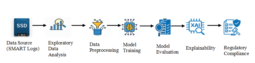
We formulate SSD failure prediction as a binary classification problem in which the objective is to predict whether an SSD will fail within a fixed 30-day prediction window. Figure 1 shows the end-to-end machine-learning pipeline for SSD failure prediction with an Explainable AI (XAI) layer. Instead of using a random train-test split, we use a temporally defined training set, walk-forward validation, and a chronologically later holdout test set to better reflect real-world deployment conditions and prevent temporal data leakage.
3.1. Data Ingestion
The first phase of the pipeline is Data Ingestion, in which SSD telemetry data (SMART logs) are collected daily at Alibaba from approximately 500,000 SSDs between January 2018 and December 2019. SMART attributes provide internal indicators of device health and are widely used in storage reliability and failure prediction research [18], [20]. Of these, 16,305 SSDs failed, while the remaining drives are considered healthy, resulting in a significant class imbalance with approximately 3% failure rate. The dataset has metadata columns (disk_id, model, ds) and SMART attributes (r_i, n_i). The r_i columns contain raw data, whereas the n_i columns contain normalized values for each attribute. In this study, we use the normalized SMART attributes (n_i) as predictive features, while metadata fields such as disk_id, model, ds, failure_time, and days_to_failure are used during preprocessing and labeling.
3.2. Exploratory Data Analysis
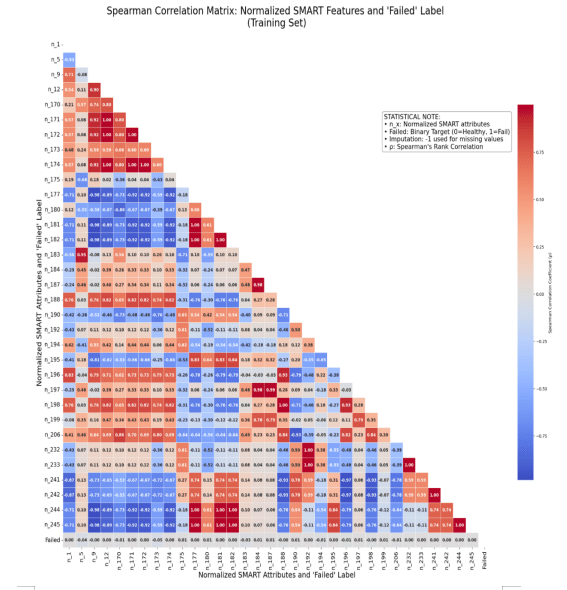
In the second phase, Exploratory Data Analysis (EDA), we looked at the differences in how healthy and failing drives behaved across six different SSD models using the temporally defined training set. Following the temporal split, we restricted this analysis to the training set to avoid leaking future data into feature selection and model design. Initial sparsity analysis indicated that 18 normalized SMART features had over 99.9% missing values and were therefore removed. For the remaining 33 normalized features, missing values were imputed with -1 to preserve the potential predictive signal of data sparsity. We intentionally used a sentinel value (-1) instead of statistical imputation so that the model could retain information about structural missingness, which may itself reflect vendor-specific SMART reporting behavior. We examined the Spearman rank correlation between normalized SMART attributes and the failure label (Failed) to identify the important indicators of degradation, as shown in Figure 2. Spearman correlation was selected because it captures monotonic relationships between SMART features and failure events without assuming linear dependencies.
Beyond direct target correlation, we examined the full feature-to-feature correlation matrix to detect multicollinearity. Our analysis revealed significant multicollinearity, with 32 redundant feature pairs having absolute Spearman correlation coefficients greater than or equal to 0.95. These correlations formed seven clusters of highly related features. Instead of applying automated feature elimination, we cross-referenced these clusters with SMART attribute definitions and retained the most operationally meaningful feature within each cluster. This cluster-based selection procedure reduced the 33 features to 17 SMART attributes while preserving the most informative degradation signals and minimizing redundancy. The final retained feature set consisted of the following 17 normalized SMART attributes: n_1, n_5, n_9, n_170, n_173, n_174, n_175, n_180, n_190, n_194, n_195, n_196, n_197, n_198, n_199, n_206, and n_232. A detailed description of the correlation clusters and the domain-informed feature selection process is provided in Appendix A.
3.3. Data Preprocessing
We built a whole preprocessing pipeline to turn the raw telemetry into a robust training set. This pipeline addressed problems with time, class imbalance, and high dimensionality:
- Temporal Filtering and Integrity:To ensure sufficient historical context, we removed all SSDs (both healthy and failed) with fewer than 30 days of operational records. Additionally, for failed drives specifically, if data gaps exceeded 30 consecutive days, we discarded records following the gap and treated the last available record as the failure date to maintain causal integrity. We created a composite key (disk_id, model) to prevent data from getting mixed up between different SSD models because disk_id is not unique across models. After this step, the dataset retained records from 101,509 unique SSDs, consisting of 16,008 failed drives and 85,501 healthy drives.
- Predictive Labeling: We created a binary target variable called “Failed” for all the SSDs by utilizing a fixed prediction window. Records that were seen within 30 days prior to a failure event were given a 1 (positive) label, while all records that came before that and all records from healthy drives were given a 0 (negative) label. At record level, the labeling process created 454,936 failed instances (Failed=1) and 54,960,816 healthy instances (Failed=0), representing 0.82% failure percentage.
- Temporal train-test split: We implemented a chronological data split to evaluate the model in a realistic deployment scenario. We identified a cut-off date (September 16, 2019), on or before which 80% of the drives failed. The 12,815 drives that failed on or before the cut-off date were reserved for the train set and 3,193 drives failed after the cut-off date were reserved for test set. The model level distribution of failed drives is follows:
Training Set (12,815 failed drives): MA1 (1,354), MA2 (819), MB1 (1,458), MB2 (542), MC1 (7,663), MC2 (979).
Test Set (3,193 failed drives): MA1 (1), MA2 (38), MB1 (310), MB2 (50), MC1 (2,664), and MC2 (130).
To create a balanced training set, we included all records from each of the 12,815 failed drives in the training set. We then sampled an equal number of healthy drives (12,815) with the same model distribution as the failed drives in the training set. For these healthy drives, all the records between January 01, 2018, and September 16, 2019, were included in the training set. Records from these healthy drives after September 16, 2019, were excluded. This resulted in a balanced training dataset containing records from 25,630 drives and 10,637,778 observations. Table 1 shows the model-wise distribution of the balanced training set.
Table 1: Model-wise distribution of the balanced training set
| Model | Number of Healthy Drives | Number of Failed Drives | Total Drives |
|---|---|---|---|
| MA1 | 1354 | 1354 | 2708 |
| MA2 | 819 | 819 | 1638 |
| MB1 | 1458 | 1458 | 2916 |
| MB2 | 542 | 542 | 1084 |
| MC1 | 7663 | 7663 | 15326 |
| MC2 | 979 | 979 | 1958 |
To create a realistic unbalanced test set, we retained records from 3,193 failed drives and 61,938 healthy drives. All the drives in test set contains the records between September 17, 2019, and December 31, 2019. So, in test set we have data from 65,131 unique drives and 5,499,337 observations. Table 2 shows the model-wise distribution of the unbalanced test dataset:
Table 2: Model-wise distribution of the unbalanced test set
| Model | Number of Healthy Drives | Number of Failed Drives | Total Drives |
|---|---|---|---|
| MA1 | 5877 | 1 | 5878 |
| MA2 | 15214 | 38 | 15252 |
| MB1 | 10084 | 310 | 10394 |
| MB2 | 12505 | 50 | 12555 |
| MC1 | 12454 | 2664 | 15118 |
| MC2 | 5804 | 130 | 5934 |
- Feature Selection and Imputation: We reduced dimensionality by removing raw SMART features (r_i) and only considering normalized features (n_i). We dropped 18 normalized attributes (n_i) that had more than 99.9% missing data. For the rest of the normalized attributes, we used a different category (-1) to impute the missing values. Finally, we used the Spearman correlation analysis from the EDA phase to get rid of 16 redundant features. This left us with a final feature set of 17 normalized SMART features.
3.4. Model Training
In the fourth phase, Model Training, we used the balanced training set produced during preprocessing to train three different tree-based ensemble models: Random Forest, XGBoost, and LightGBM. These algorithms were selected because tree-based ensembles are well suited to high-dimensional telemetry data and have demonstrated strong performance in prior storage failure prediction studies [2], [20].
We used temporally balanced train set for model development. To perform hyperparameter tuning while retaining chronological order, we used fixed-date walk-forward validation on the training data. We defined three validation folds using temporal cutoffs on January 1, 2019, March 1, 2019, and May 1, 2019, with a 60-day validation window after each cutoff. To prevent drive-level leakage, any drive appearing in the training portion of a fold was excluded from the corresponding validation fold. This ensured both temporal integrity and drive-level isolation.
We used Randomized Search Cross-Validation to perform hyperparameter tuning for XGBoost, LightGBM, and Random Forest. The search spaces for the evaluated hyperparameters are summarized in Table 3. Randomized search was performed using multiple parameter combinations with cross-validation on the temporally defined training set to identify configurations that maximize predictive performance while maintaining generalization. The final hyperparameter configurations selected for each model, cost ratio, and validation fold are reported in Table 4. Notably, the selected configurations were largely consistent across different cost ratios, indicating that performance variation is primarily driven by threshold optimization rather than substantial changes in model structure.
Table 3: Hyperparameter Search Space Used in Randomized Search
| Model | Hyperparameter | Search Space |
|---|---|---|
| XGBoost | max_depth | {3, 5, 7, 9} |
| learning_rate | {0.01, 0.05, 0.1, 0.2} | |
| n_estimators | {100, 300, 500} | |
| min_child_weight | {1, 5, 10} | |
| gamma | {0, 0.1, 0.2} | |
| scale_pos_weight | {IR, 1.5 × IR, 2 × IR} | |
| subsample | {0.7, 0.8, 1.0} | |
| colsample_bytree | {0.7, 0.8, 1.0} | |
| LightGBM | n_estimators | {100, 300, 500} |
| learning_rate | {0.01, 0.05, 0.1} | |
| num_leaves | {31, 63, 127} | |
| scale_pos_weight | {IR, 1.5 × IR} | |
| Random Forest | n_estimators | {100, 300} |
| max_depth | {5, 10, 20} | |
| min_samples_split | {2, 10} | |
| class_weight | {balanced, balanced_subsample} |
IR denotes the class imbalance ratio (number of healthy samples divided by failed samples).
Table 4: Final Hyperparameters Selected After Randomized Search
| Model | Cost Ratio (FN: FP) | Fold | Best Hyperparameters |
|---|---|---|---|
| XGBoost | 10:1 | 1 | subsample=0.8, scale_pos_weight=56.18, n_estimators=100, min_child_weight=10, max_depth=5, learning_rate=0.1, gamma=0.2, colsample_bytree=0.8 |
| 10:1 | 2 | subsample=0.8, scale_pos_weight=56.18, n_estimators=100, min_child_weight=1, max_depth=3, learning_rate=0.01, gamma=0.1, colsample_bytree=0.8 | |
| 10:1 | 3 | subsample=0.8, scale_pos_weight=56.18, n_estimators=100, min_child_weight=10, max_depth=5, learning_rate=0.1, gamma=0.2, colsample_bytree=0.8 | |
| 25:1 | 1-3 | Same as 10:1 configuration | |
| 50:1 | 1-3 | Same as 10:1 configuration | |
| 100:1 | 1-3 | Same as 10:1 configuration | |
| LightGBM | 50:1 | 1 | scale_pos_weight=28.09, num_leaves=31, n_estimators=500, learning_rate=0.01 |
| 50:1 | 2-3 | scale_pos_weight=42.14, num_leaves=31, n_estimators=100, learning_rate=0.05 | |
| Random Forest | 50:1 | 1-2 | n_estimators=100, min_samples_split=2, max_depth=5, class_weight=balanced |
| 50:1 | 3 | n_estimators=100, min_samples_split=2, max_depth=10, class_weight=balanced_subsample |
3.5. Model Evaluation
In the fifth phase, Model Evaluation, we moved beyond standard statistical metrics to evaluate performance in a real-world operational context. We calculated Precision, Recall, F1-score, ROC-AUC, and PR-AUC, with a focus on Recall, false alarm rate (FAR), and cost-sensitive threshold performance because SSD failure prediction is a highly imbalanced classification problem [20], [25].
For each validation fold, the decision threshold was optimized over a range of candidate thresholds to minimize operational cost. We selected the final model using a custom Operational Cost Function. This function assigns a significantly higher cost to missed failures (False Negatives) than to false alarms (False Positives). The total cost is calculated as:
$$
\text{Total Cost} = (FP \times \text{\$}10) + (FN \times \text{\$}500) \tag{1}
$$
Here, a False Negative (FN) incurs a $500 penalty to reflect the risks of service disruption and data loss, while a False Positive (FP) incurs a $10 cost for unnecessary inspection labor. The 50:1 cost ratio represents an illustrative operating scenario in which missing an impending failure is substantially more expensive than a precautionary inspection. To test the robustness of this assumption, we also conducted cost-sensitivity analysis across different false-negative to false-positive ratios of 10:1, 25:1, 50:1, and 100:1.
The final holdout test set was then used for one-time evaluation of the selected model after retraining on the full training data with the best hyperparameters.
3.6. Explainability and Regulatory Compliance
We added a post-hoc explainability layer directly to the prediction pipeline to meet the transparency requirements discussed in Section 2.1. We used LIME [4] to generate local surrogate models for each failure alert, which let operators interpret specific predictions by identifying the SMART attributes that contributed most to the decision. At the same time, SHAP values [5] were computed to provide a global view of feature importance and to verify that the model’s decision patterns align with known physical degradation signals instead of false correlations. Unlike prior work that applies explainability primarily for diagnostic interpretation, our approach explicitly integrates these methods within an operational monitoring pipeline to support auditability and decision transparency in production environments.
In addition to interpretability, we analyzed model behavior at both global and local levels using SHAP and LIME, respectively. While SHAP provided a global view of feature importance across the dataset, LIME enabled instance-level inspection of individual predictions, allowing us to validate that the model’s decisions are consistent with known SSD degradation characteristics. This dual-level explanation supports both system-level and instance-level validation, which are essential for compliance with AI governance requirements. This setup turns opaque probability scores into clear insights that can be verified, which directly supports the transparency standards set by frameworks like the NIST AI Risk Management Framework [15].
3.7. Data and Code Availability
The original SSD dataset used in this study is publicly available as part of the Alibaba DCBrain SSD SMART logs repository: https://github.com/alibaba-edu/dcbrain/tree/master/ssd_smart_logs
The code used for data preprocessing, model training, cost-sensitive evaluation, calibration analysis, ablation study, per-model analysis, and explainability analysis is publicly available at: https://github.com/sauravintheocean/SSD_Failure_Prediction_XAI
Due to the large size of the dataset, the processed data is not distributed directly. However, the repository includes all necessary scripts and documentation to reconstruct the processed dataset and reproduce the results reported in this paper.
4. Results and Analysis
In this section, we present the experimental results of our research, focusing on predictive performance, operational cost, and explainability under the temporal validation method described in Section 3. First, we analyze the sensitivity of the XGBoost model to different false-negative to false-positive cost ratios (10:1, 25:1, 50:1, 100:1). This analysis evaluates how the optimal decision threshold and model performance vary under different cost assumptions and to identify an appropriate operating regime for failure prediction. Based on this analysis, the 50:1 cost ratio was selected as the most suitable trade-off between minimizing total operational cost and maximizing recall of impending failures. Second, we compare the performance of Random Forest, XGBoost, and LightGBM using walk-forward validation under the selected 50:1 cost ratio. Finally, we report the performance of the final retrained XGBoost model on the chronologically later holdout test set and assess its transparency using SHAP and LIME.
4.1. Cost Sensitivity Analysis of XGBoost
Table 5 reports the mean and standard deviation across the three temporal validation folds. As the cost ratio increased from 10:1 to 50:1, the mean recall of XGBoost increased from 44.69% ± 48.11% to 70.83% ± 50.52%, while the mean false alarm rate increased from 0.3595 ± 0.5553 to 0.6686 ± 0.5674. The optimal average threshold decreased from 0.4700 ± 0.3984 at the lower cost ratios to 0.3114 ± 0.3532 at the higher ratios, indicating that the observed changes are primarily driven by threshold adjustment rather than substantial changes in model structure.
Although variability across folds is substantial, this is largely due to the highly uneven number of failure cases in the validation windows. The fold-level results should therefore be interpreted as an exploratory sensitivity analysis rather than as a definitive estimate of deployment variance.
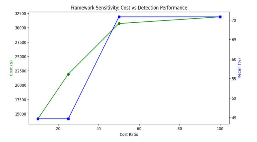
Increasing the cost ratio beyond 50:1 did not lead to any improvement in recall, precision, or ranking performance. As shown in Table 5, the performance metrics at 50:1 and 100:1 are identical, while the mean operational cost increases from $30,720 to $31,886.67. This indicates that the model has already reached its maximum achievable recall under the given feature space and temporal validation setup. Therefore, the 50:1 ratio represents the most cost-effective operating point, achieving the same detection performance as higher ratios while avoiding unnecessary increases in operational cost.
Table 5: XGBoost Cost-Sensitivity Analysis Across Temporal Validation Folds
| Cost Ratio (FN: FP) | Mean Cost ($) ± SD | Avg. Recall ± SD | Avg. Precision ± SD | Avg. FAR ± SD | Avg. PR-AUC ± SD | Avg. ROC-AUC ± SD | Avg. Threshold ± SD |
|---|---|---|---|---|---|---|---|
| 10:1 | 14106.67 ± 11476.05 | 44.69% ± 48.11% | 7.36% ± 3.21% | 0.3595 ± 0.5553 | 0.0457 ± 0.0337 | 0.4914 ± 0.1171 | 0.4700 ± 0.3984 |
| 25:1 | 21906.67 ± 19790.86 | 44.69% ± 48.11% | 7.36% ± 3.21% | 0.3595 ± 0.5553 | 0.0457 ± 0.0337 | 0.4914 ± 0.1171 | 0.4700 ± 0.3984 |
| 50:1 | 30720.00 ± 32134.99 | 70.83% ± 50.52% | 5.41% ± 3.78% | 0.6686 ± 0.5674 | 0.0457 ± 0.0337 | 0.4914 ± 0.1171 | 0.3114 ± 0.3532 |
| 100:1 | 31886.67 ± 30698.22 | 70.83% ± 50.52% | 5.41% ± 3.78% | 0.6686 ± 0.5674 | 0.0457 ± 0.0337 | 0.4914 ± 0.1171 | 0.3114 ± 0.3532 |
Figure 3 illustrates the sensitivity of the final XGBoost model to varying cost ratios. As the cost ratio increases, the model prioritizes higher recall, resulting in more aggressive failure detection at the expense of increased false alarms. This behavior highlights the trade-off between minimizing missed failures and controlling operational overhead in real-world data center environments.
4.2. Model Comparison at 50:1 Cost Ratio
We compared the performance of XGBoost, LightGBM, and Random Forest at a 50:1 cost ratio using walk-forward temporal validation. Table 6 reports the mean and standard deviation across the three validation folds.
Table 6: Model Comparison at 50:1 Cost Ratio (Mean ± SD)
| Model | Mean Cost ($) ± SD | Avg. Recall ± SD | Avg. Precision ± SD | Avg. FAR ± SD | Avg. PR-AUC ± SD | Avg. ROC-AUC ± SD | Avg. Threshold ± SD |
|---|---|---|---|---|---|---|---|
| XGBoost | 30720.00 ± 32134.99 | 70.83% ± 50.52% | 5.41% ± 3.78% | 0.6686 ± 0.5674 | 0.0457 ± 0.0337 | 0.4914 ± 0.1171 | 0.3114 ± 0.3532 |
| LightGBM | 30763.33 ± 32213.80 | 70.83% ± 50.52% | 5.41% ± 3.79% | 0.6691 ± 0.5679 | 0.0535 ± 0.0374 | 0.5738 ± 0.1938 | 0.3272 ± 0.2839 |
| Random Forest | 30886.67 ± 32411.74 | 70.83% ± 50.52% | 5.41% ± 3.79% | 0.6711 ± 0.5696 | 0.0453 ± 0.0358 | 0.4377 ± 0.1140 | 0.3114 ± 0.3376 |
All three models achieved identical mean recall (70.83% ± 50.52%), which indicates that under aggressive cost-sensitive thresholding, each model prioritizes maximizing failure detection. However, differences emerge in ranking performance and stability. LightGBM achieved the highest ROC-AUC (0.5738 ± 0.1938), followed by XGBoost and Random Forest. Also, XGBoost achieved slightly lower false alarm rates and competitive precision compared to both baselines. Despite these differences, the overall performance across models remains highly similar. The large standard deviations observed across all metrics are primarily due to the uneven distribution of failure cases across validation folds, particularly the presence of folds with very few failure instances.
To further assess whether the observed differences are statistically significant, we conducted paired t-tests and Wilcoxon signed-rank tests using fold-level results. As shown in Table 7, no statistically significant differences were observed between XGBoost and the baseline models for cost, recall, precision, FAR, PR-AUC, or F1-score (p > 0.05). A statistically significant difference was observed only for ROC-AUC between XGBoost and Random Forest (p = 0.025), indicating improved ranking performance for XGBoost in this specific comparison.
Table 7: Statistical Significance Tests (XGBoost vs Baselines, 50:1)
| Comparison | Metric | p-value (t-test) | Significance |
|---|---|---|---|
| XGBoost vs LightGBM | Cost | 0.465 | Not significant |
| Recall | Identical | ||
| Precision | 0.856466 | Not significant | |
| FAR | 0.557347 | Not significant | |
| PR_AUC | 0.231781 | Not significant | |
| ROC_AUC | 0.307106 | Not significant | |
| F1 | 0.808505 | Not significant | |
| XGBoost vs Random Forest | Cost | 0.422650 | Not significant |
| Recall | |||
| Precision | 0.422650 | Not significant | |
| FAR | 0.422650 | Not significant | |
| PR_AUC | 0.826461 | Not significant | |
| ROC_AUC | 0.025055 | Significant | |
| F1 | 0.422650 | Not significant |
These results indicate that all three models perform comparably under cost-sensitive thresholding, with most performance differences not statistically significant. While XGBoost demonstrates competitive performance and slightly improved ranking behavior in specific comparisons, the results suggest that model choice has a limited impact relative to threshold optimization in this setting.
4.3. Final Model Evaluation on Holdout Test Set
We retrained the XGBoost model on the complete training dataset using the optimal hyperparameters identified in Section 3.4 at the selected 50:1 cost ratio. The final model was evaluated on a chronologically later holdout test set to simulate real-world deployment conditions. Instead of using a fixed classification threshold, we performed a threshold sweep on the holdout set to identify the operating point that maximizes economic benefit. The optimal threshold was found to be 0.68, which balances missed failures and false alarms under the defined cost structure. Table 8 shows the performance of XGBoost on the holdout test set.
Table 8: Final model performance on holdout test set
| Metric | Value |
|---|---|
| Cost Ratio (FN: FP) | 50:1 |
| Optimal Threshold | 0.68 |
| Net Operational Savings | $13,419,280 |
| Recall | 67.98% |
| Precision | 4.43% |
| F1-score | 0.083 |
| FAR | 0.1878 |
| PR-AUC | 0.0386 |
| ROC-AUC | 0.7625 |
| TP | 47,236 |
| FP | 1,019,872 |
| FN | 22,250 |
| TN | 4,409,979 |
The model successfully identified 67.98% of impending failures, while maintaining a manageable false alarm rate (FAR = 0.1878). Although precision remains low (4.43%), this behavior is expected in highly imbalanced failure prediction tasks where maximizing recall is critical. The higher ROC-AUC observed on the holdout test set compared to validation folds is primarily due to the larger number of failure instances, resulting in a more stable and representative estimate of ranking performance.
From an operational perspective, the model generated approximately 22.6 alerts per true failure, reflecting the trade-off between proactive failure detection and inspection overhead. Despite this, the optimized strategy yields a substantial net operational savings of $13.4 million, demonstrating the economic value of cost-sensitive learning in data center environments. While the proposed model achieves significant reductions in missed failures, it generates many false alarms (approximately 1.02 million in the holdout period). In practice, data centers do not manually inspect every flagged drive. Instead, alerts are typically integrated into automated monitoring pipelines and prioritized using additional operational heuristics.
First, alerts can be ranked by predicted failure probability, allowing operators to focus only on the top-k% highest-risk drives. This prioritization can substantially reduce inspection overhead while still capturing a large proportion of true failures. Second, many false positives correspond to drives exhibiting early signs of degradation that may not immediately fail but still warrant closer monitoring. As a result, these alerts are not necessarily wasted effort but can contribute to preventive maintenance strategies. Third, inspection in modern data centers is often partially automated, involving background diagnostics, SMART log analysis, or scheduled maintenance cycles rather than manual intervention for each alert. Therefore, the reported number of false alarms should be interpreted as an upper bound under a fully reactive scenario. In practice, alert prioritization, batching, and automation significantly reduce the effective operational burden.
4.4. Ablation Study
To quantify the contribution of different feature groups, we conducted an ablation study by systematically removing key categories of SMART attributes, including wear indicators, temperature-related features, and error metrics. The results are summarized in Table 9.Removing wear-related features (n_173 and n_180) resulted in a dramatic performance degradation, with recall dropping from 67.98% to 7.85% and F1-score decreasing from 0.083 to 0.017. This confirms that wear-level indicators are the dominant predictors of SSD failure and are critical for reliable detection. In contrast, removing temperature-related features (n_190 and n_194) led to a moderate reduction in recall (67.98% to 61.05%), indicating that thermal signals provide complementary information that improves model robustness but are not the primary drivers of prediction. Finally, removing error-related features had minimal impact on recall but slightly reduced precision and increased the false alarm rate, suggesting that these features contribute marginally to decision refinement but are less informative than wear and temperature indicators.Overall, the ablation results are consistent with the SHAP analysis and demonstrate that the model’s predictions are grounded in physically meaningful degradation signals rather than spurious correlations. All ablation experiments were conducted on the holdout test set using the fixed optimal threshold (T = 0.68) to ensure fair comparison.
Table 9: Ablation Study Results
| Experiment | Recall | Precision | F1 | FAR |
|---|---|---|---|---|
| Full Model | 67.98% | 4.43% | 0.083 | 0.1878 |
| No Wear Features | 7.85% | 0.98% | 0.017 | 0.1017 |
| No Temperature | 61.05% | 4.54% | 0.084 | 0.1643 |
| No Error Metrics | 68.97% | 4.16% | 0.084 | 0.2036 |
4.5. Calibration Analysis
To evaluate the reliability of predicted probabilities, we assessed model calibration using a reliability diagram, calibration table, and Brier score on the holdout test set. As shown in Figure 4, the reliability curve lies consistently below the diagonal, indicating that predicted probabilities systematically overestimate the true failure likelihood, particularly at higher probability ranges. The calibration was evaluated post hoc and was not explicitly optimized during model training.
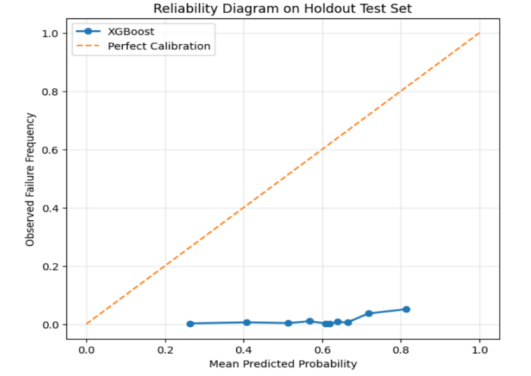
This trend is further supported by the calibration table (Table 10), where observed failure frequencies remain significantly lower than predicted probabilities across all bins.
Table 10: Calibration Table
| Predicted Probability Bin | Observed Frequency |
|---|---|
| 0.265 | 0.0024 |
| 0.408 | 0.0062 |
| 0.514 | 0.0036 |
| 0.568 | 0.0102 |
| 0.608 | 0.0026 |
| 0.619 | 0.0008 |
| 0.639 | 0.0078 |
| 0.665 | 0.0061 |
| 0.717 | 0.0365 |
| 0.814 | 0.0513 |
The Brier score of 0.3547 indicates limited probability calibration, which is expected given the extreme class imbalance and the cost-sensitive optimization strategy employed in this work. The model is explicitly optimized to maximize recall and economic utility rather than to produce well-calibrated probability estimates. Despite this, threshold-based decision making remains effective, as the framework relies on relative risk ranking rather than absolute probability accuracy. The optimal operating threshold is determined empirically through cost optimization, ensuring robust operational performance even in the presence of calibration error. Despite calibration limitations, the model maintains strong ranking performance (ROC-AUC = 0.7625), indicating reliable relative risk ordering. Future work may explore post-hoc calibration techniques such as Platt scaling or isotonic regression to improve probability reliability without compromising cost-sensitive performance.
4.6. Baseline Comparison (Walk-Forward Validation)
To further evaluate the effectiveness of the proposed framework, we compared its performance against three additional baseline approaches: (1) Logistic Regression, (2) a heuristic top-k model based on wear-level indicators, and (3) a feature-reduced XGBoost model inspired by prior work. All models were evaluated using the same walk-forward temporal validation and cost-sensitive optimization framework (50:1 cost ratio). The results are summarized in Table 11.
Logistic Regression achieves high recall in some folds but only by significantly increasing the false alarm rate, indicating poor discrimination capability under extreme class imbalance. In contrast, the heuristic top-k baseline demonstrates limited predictive power, with substantially lower recall and higher operational cost, confirming that simple threshold-based rules are insufficient for SSD failure prediction. The feature-reduced XGBoost baseline performs better than the heuristic model but exhibits instability across folds. But all baseline models failed to detect failures in Fold 2, where only eight failure events were present. Under such extreme sparsity, cost minimization favors conservative thresholds, leading to zero recall. This highlights the sensitivity of simpler models to rare-event scenarios.
Finally, these results indicate that accurate SSD failure prediction requires modeling complex, multi-dimensional feature interactions. Simplified models and heuristic approaches are insufficient for capturing the underlying failure dynamics in hyperscale environments.
Table 11: Baseline Comparison at 50:1 Cost Ratio (Mean ± SD)
| Model | Mean Cost ($) ± SD | Avg. Recall ± SD | Avg. Precision ± SD | Avg. FAR ± SD | Avg. PR-AUC ± SD | Avg. ROC-AUC ± SD | Avg. Threshold ± SD |
|---|---|---|---|---|---|---|---|
| Logistic Regression | 26,920 ± 25,946 | 66.67% ± 57.7% | 4.42% ± 5.05% | 0.60 ± 0.53 | 0.088 ± 0.113 | 0.515 ± 0.257 | 0.3669 ± 0.3356 |
| Heuristic Top-k | 44,233 ± 40,508 | 33.07% ± 39.3% | 4.74% ± 5.43% | 0.29 ± 0.36 | 0.090 ± 0.127 | 0.505 ± 0.182 | 0.2955 ± 0.3601 |
| Xu-style XGBoost | 30,310 ± 31,531 | 66.67% ± 57.7% | 4.25% ± 5.12% | 0.65 ± 0.56 | 0.085 ± 0.107 | 0.524 ± 0.170 | 0.4224 ± 0.1995 |
4.7 Final Holdout Comparison
We compared the performance of proposed XGBoost model against the strongest baseline models on an independent holdout test set. Logistic Regression and the feature-reduced XGBoost model were selected based on their performance in the walk-forward validation stage. The results are summarized in Table 12. Logistic Regression has extremely low recall (0.7%), failing to detect most failures despite maintaining a low false alarm rate. This indicates that linear models are insufficient for capturing the complex, non-linear degradation patterns present in SSD data.
The feature-reduced Xu-style XGBoost achieves the highest recall (72.67%) and lowest operational cost ($18.51M), resulting in the highest net savings ($16.24M). It also produces fewer alerts per true failure (18.8), indicating improved operational efficiency. This improvement is due to focusing on a subset of highly predictive SMART attributes, reducing noise from less informative features. However, this simplified model demonstrates reduced robustness, as evidenced by its instability during walk-forward validation.
The full-feature XGBoost model achieves slightly lower recall (67.98%) and higher operational cost but demonstrates more stable performance across temporal validation (Section 4.6). These results highlight an important trade-off between model simplicity and robustness. While feature reduction can improve performance on specific datasets, the proposed framework prioritizes consistent, cost-sensitive performance across diverse operating conditions.
Table 12: Final Holdout Comparison (50:1) comparison
| Model | Optimal Threshold | Net Savings ($) | Cost ($) | Recall | Precision | F1 | FAR | PR-AUC | ROC-AUC | Alerts/Failure |
|---|---|---|---|---|---|---|---|---|---|---|
| XGBoost (Full) | 0.68 | 13.4M | 21.32M | 67.98% | 4.43% | 0.083 | 0.188 | 0.039 | 0.7625 | 22.6 |
| Logistic Regression | 0.85 | 0.11M | 34.63M | 0.70% | 3.61% | 0.0117 | 0.002 | 0.015 | 0.582 | 27.7 |
| Xu-style XGBoost | 0.53 | 16.2M | 18.51M | 72.67% | 5.31% | 0.0989 | 0.166 | 0.044 | 0.768 | 18.8 |
4.8 Per-Model Performance Analysis
To evaluate model generalization across different hardware types, we analyzed performance separately for each SSD model on the holdout test set. The results are summarized in Table 13.
Table 13: Per-Model Performance Analysis
| Model | Samples | Recall | Precision | FAR |
|---|---|---|---|---|
| MA1 | 481,617 | 8.00% | 0.01% | 0.0340 |
| MA2 | 1,252,002 | 6.73% | 0.12% | 0.0422 |
| MB1 | 927,930 | 29.22% | 1.73% | 0.1323 |
| MB2 | 1,127,559 | 7.69% | 0.08% | 0.1063 |
| MC1 | 1,189,688 | 74.53% | 7.06% | 0.4945 |
| MC2 | 520,541 | 81.66% | 1.57% | 0.2878 |
The model demonstrates substantial variation in predictive performance across SSD models. For example, MC2 and MC1 exhibit strong recall (81.66% and 74.53%, respectively), indicating that failure patterns for these models are well captured by the learned feature space. In contrast, other models such as MA1, MB2, and MA2 show significantly lower recall (below 10%), suggesting that their failure signatures are either less pronounced or not fully represented by the available SMART attributes. This variability highlights the heterogeneous nature of SSD failure mechanisms across different hardware models. Some devices exhibit clear degradation patterns (e.g., wear-out behavior), while others may fail due to more stochastic or unobserved factors, making prediction inherently more challenging. Despite these differences, high-performing models contribute significantly to overall cost savings. From an operational perspective, this suggests that model deployment can be further optimized by incorporating model-specific thresholds or training specialized models per device family.
These findings emphasize the importance of hardware-aware modeling strategies and motivate future work on domain adaptation and per-device calibration techniques. This result further reinforces that global performance metrics may mask significant variability across hardware types.
4.9. Explainability Analysis
To ensure the model’s decisions are transparent and trustworthy for data center operators, we applied SHAP for global feature analysis and LIME for individual failure auditing.
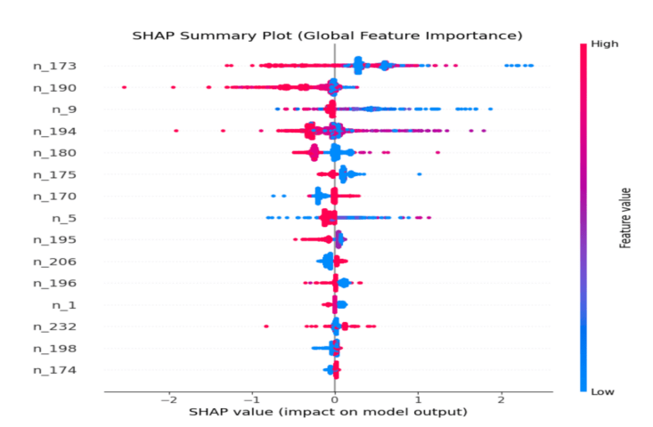
Global Feature Importance (SHAP)
Features are ranked by their mean absolute SHAP value, with color representing the feature value (red = high, blue = low). As shown in Figure 5, n_173 (Wear Leveling Count) emerges as the most important feature. Lower values of n_173 (blue points) are strongly associated with positive SHAP values, indicating higher failure risk. This behavior is consistent with the physical interpretation of wear leveling, where lower values of the normalized wear-leveling count indicate progressive exhaustion of SSD endurance.
In addition, n_190 (Airflow Temperature / thermal variation indicator), n_9 (Power-On Hours), n_194 (Temperature), and n_180 (Unused Reserved Block Count) also contribute to the model’s predictions, capturing complementary signals related to device aging, thermal stress, and available spare capacity. The SHAP distributions show consistent directional patterns across these features, where variations in feature values correspond to predictable changes in failure risk.
This indicates that the XGBoost model is learning meaningful hardware-level signals rather than spurious correlations, supporting its reliability for real-world deployment.
Local Failure Diagnosis (LIME)
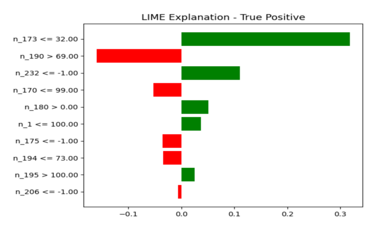
We used LIME analysis to audit individual predictions, which gave us detailed information about each prediction.
Figure 6 illustrates a True Positive prediction for a failed drive. The LIME explanation shows that n_173 (Wear Leveling Count) is the dominant contributor, where very low values strongly push the prediction toward failure. Additional contributing factors include n_180 (Unused Reserved Block Count) and imputed values such as n_232 ≤ -1, indicating potential degradation or missing telemetry signals associated with increased failure risk. These features collectively reinforce the model’s ability to detect drives nearing end-of-life conditions.
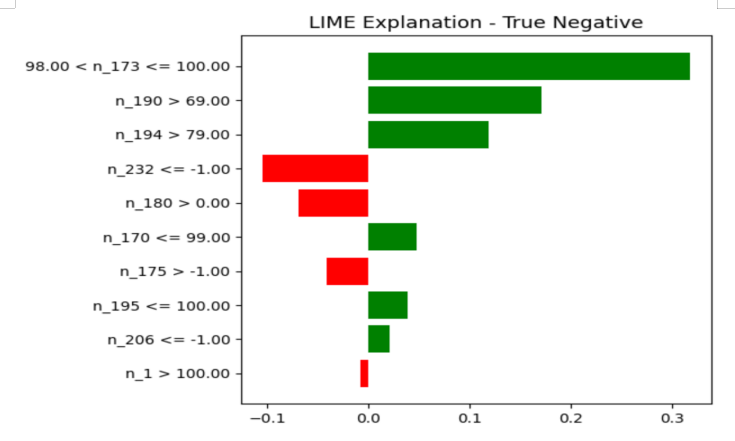
Conversely, Figure 7 presents a True Negative prediction for a healthy drive. In this case, high values of n_173 (Wear Leveling Count) are the primary contributors toward a healthy classification, indicating sufficient remaining endurance. Additional positive contributions from n_190 (thermal indicator) and n_194 (temperature) further support the healthy prediction. While some features (e.g., imputed or weak degradation signals) push slightly toward failure, their influence is outweighed by stronger indicators of normal operating conditions.
These instance-level explanations demonstrate that the model’s predictions are driven by coherent and interpretable feature interactions, consistent with known physical behavior of SSD degradation and operational conditions.
5. Discussion
In this section, we interpret the experimental results within the broader context of data center operations. Beyond standard performance metrics, we analyze the operational feasibility of the proposed framework, justify the economic trade-offs inherent in the “Safety-First” strategy, and discuss the long-term reliability implications for hyperscale storage fleets.
5.1. Implications for Data Center Operations
The results show that under cost-sensitive thresholding, all three models (XGBoost, LightGBM, and Random Forest) converge to similar operating characteristics, achieving comparable recall (~70%) and cost performance. This indicates that threshold optimization plays a more significant role than model architecture in highly imbalanced failure prediction settings.
Despite similar aggregate performance, XGBoost was selected as the final model due to its consistent behavior across validation folds, competitive false alarm rates, and strong interpretability properties. The SHAP and LIME analyses further confirm that its predictions are driven by physically meaningful signals, making it more suitable for operational deployment.
From an operational perspective, the proposed framework functions as a high-sensitivity screening system rather than an autonomous decision-maker. The deployment workflow follows a two-stage process:
- The model flags drives exhibiting anomalous behavior (e.g., degradation in wear-leveling count or abnormal thermal patterns).
- Flagged drives are subjected to lightweight diagnostics, SMART log inspection, or scheduled maintenance review.
This hierarchical approach ensures that false alarms incur low marginal cost, while significantly reducing the risk of catastrophic failures. As a result, the system enables a transition from reactive to proactive maintenance strategies in large-scale storage environments.
An important observation from the baseline comparison is the trade-off between model simplicity and robustness. While the feature-reduced Xu-style XGBoost achieves higher recall and lower cost on the holdout set, it exhibits instability across temporal validation folds. In contrast, the full-feature XGBoost model provides more consistent performance, highlighting the importance of robustness in real-world deployment scenarios.
5.2. Economic Impact and Cost Asymmetry
The primary driver of this study is the asymmetric nature of failure costs. Missing a failure (false negative) can lead to severe consequences, including data loss and service disruption, while false alarms primarily incur inspection costs. Through cost-sensitivity analysis (Section 4.1), we observed that increasing the FN:FP ratio shifts the model toward higher recall at the expense of increased false alarms. Also, performance stabilizes beyond a 50:1 ratio, where further increases do not improve recall or ranking metrics but lead to higher operational cost. This identifies 50:1 as the most cost-effective operating point.
On the holdout test set, the optimized model achieved $13.4 million in net operational savings, demonstrating the economic value of cost-aware threshold selection. This highlights a key insight: In hyperscale environments, optimal decision-making is driven by economic objectives rather than traditional classification metrics.
5.3. The Strategic importance of Low Precision
A key finding of this study is that low precision (~4.4%) is not a limitation but a deliberate design choice under asymmetric cost conditions. In conventional classification tasks, low precision is undesirable. However, in failure prediction:
- Missing failures is extremely costly
- False alarms are relatively inexpensive
Thus, maximizing precision would require stricter thresholds, significantly reducing recall and increasing the risk of undetected failures. Instead, the proposed framework adopts a “Safety-First” strategy, prioritizing recall to ensure that most at-risk drives are identified. Importantly, the explainability analysis confirms that false positives are not random noise; rather, they often correspond to drives exhibiting early warning signals such as thermal stress or wear degradation.
These drives, although not immediately failing, represent latent risk, making their identification operationally valuable. Consequently, the model functions as a preventive screening mechanism, balancing reliability and operational cost.
5.4. Managing False Alarms
A practical challenge in deployment is the high number of false alarms (approximately 1.02 million in the holdout period). However, in real-world data center environments, not all alerts are treated equally.
Following strategies help mitigate this burden:
- Risk-based prioritization: Alerts can be ranked by predicted failure probability, allowing operators to focus on the highest-risk subset (e.g., top 5–10%).
- Batching and automation: Many diagnostics are automated through SMART monitoring tools, reducing manual inspection effort.
- Preventive maintenance value: Some false positives correspond to drives under stress that may fail soon, providing early intervention opportunities.
Therefore, the reported false alarm count represents a worst-case upper bound, while the effective operational burden is significantly lower in practice.
5.5. Limitations and Future Directions
This research highlights the limitations that are inherent to the current methodology:
- Temporal Resolution: The current analysis relies on daily snapshots of SMART attributes and the current data frequency works well for capturing slow degradation (like wear leveling), but it makes it hard to detect “rapid-onset” failures, which are catastrophic breakdowns that develop and strike within the 24-hour interval between status updates (such mechanical shock or controller failure).
- Dataset Specificity:The Alibaba dataset is enormous, but it represents a specific kind of operating environment with distinct patterns of workload and cooling strategies. As a result, the model’s applicability to other hyperscale data centers or to storage fleets characterized by different drive manufacturers and model generations requires additional validation.
- Cost Model Simplification: Although we conducted sensitivity analysis across four false-negative to false-positive cost ratios (10:1, 25:1, 50:1, and 100:1), these scenarios remain predefined and illustrative. In operational settings, the true cost of missed failures and false alarms may vary dynamically depending on data criticality, drive type, service-level requirements, and replacement logistics.
- Explainability vs. Causality:SHAP and LIME identify correlations (e.g., high temperature correlates with failure), but they can’t show that one thing causes another. It is still unclear if the temperature caused the failure or if a failing mechanical part produced the extra heat.
Based on these limitations, we propose the following avenues for future research:
- Integration of Time-Series Deep Learning Models:Moving from static classifiers like XGBoost to sequence-based models, such as Long Short-Term Memory (LSTM) networks or Transformers, enables explicit modeling of the rate of change of SMART characteristics, possibly improving the capture of rapid degradation events.
- Heterogeneous Fleet Validation:Extending the framework to include Hard Disk Drives (HDDs). Mechanical storage exhibits fundamentally different failure modes than flash-based SSDs (e.g., motor vibration vs. NAND wear), requiring distinct feature engineering and failure signatures to ensure the framework generalizes across a mixed data center fleet.
- Dynamic Cost Functions:Developing an adaptive thresholding system that changes the decision boundary in real time based on how important the data is and how much it costs to replace the drive, instead of using a fixed global constant.
- Human-in-the-Loop Evaluation: Conducting field studies with data center technicians to evaluate the interpretability and actionability of LIME explanations. Feedback from domain experts is crucial to refining the visualization of risk factors for non-data scientists, ensuring that model outputs build trust and facilitate correct decision-making.
6. Conclusion
This study demonstrates that effective predictive maintenance in hyperscale data centers requires moving beyond standard accuracy metrics toward cost-sensitive and explainable AI frameworks. Using the Alibaba SSD dataset, we addressed the extreme class imbalance in failure prediction by combining cost-aware threshold optimization with interpretable modeling techniques.
Our results show that model performance in this setting is driven less by algorithmic differences and more by cost-sensitive threshold selection. Through systematic sensitivity analysis across multiple cost ratios (10:1, 25:1, 50:1, and 100:1), we identified 50:1 as the most cost-effective operating point, beyond which no further improvements in recall or ranking performance were observed.
On a chronologically separated holdout test set, the optimized XGBoost model achieved 67.98% recall and generated approximately $13.4 million in net operational savings, demonstrating the practical value of a “Safety-First” strategy that prioritizes failure detection over precision. While this approach results in a higher number of false alarms, we show that these can be effectively managed through prioritization, automation, and staged inspection workflows, making the framework operationally feasible.
Importantly, the integration of SHAP and LIME ensures that model predictions are transparent and physically interpretable, with key features such as wear leveling, thermal indicators, and device age aligning with known hardware degradation mechanisms. This interpretability is critical for building trust and enabling adoption in real-world data center environments.
Although the proposed framework demonstrates strong performance, it remains subject to limitations related to dataset specificity, temporal resolution, and simplified cost modeling. Future work should focus on extending the approach to time-series deep learning models, validating across heterogeneous storage fleets, and incorporating adaptive, context-aware cost functions.
Ultimately, this research bridges the gap between predictive modeling and operational deployment. By aligning machine learning objectives with economic realities and providing interpretable decision support, the proposed framework offers a scalable solution for reliability management not only in data centers but also in other critical infrastructure domains where failure costs are asymmetric, and transparency is essential.
- D. Reinsel, J. Gantz, J. Rydning, “The digitization of the world from edge to core”, Tech. Rep. US44413318, IDC, 2018.
- F. Xu, S. Han, P. P. C. Lee, Y. Liu, C. He, J. Liu, “General feature selection for failure prediction in large-scale ssd deployment”, “2021 51st Annual IEEE/IFIP International Conference on Dependable Systems and Networks (DSN)”, pp. 263–270, 2021, https://doi.org/10.1109/DSN48987.2021.00039.
- J. Sevilla, L. Heim, A. Ho, T. Besiroglu, M. Hobbhahn, P. Villalobos, “Compute trends across three eras of machine learning”, “2022 International Joint Conference on Neural Networks (IJCNN)”, pp. 1–8, 2022, https://doi.org/10.1109/IJCNN55064.2022.9891914.
- S. Maneas, K. Mahdaviani, T. Emami, B. Schroeder, “A study of SSD reliability in large scale enterprise storage deployments”, “18th USENIX Conference on File and Storage Technologies (FAST 20)”, pp. 137–149, USENIX Association, Santa Clara, CA, 2020.
- M. T. Ribeiro, S. Singh, C. Guestrin, “Why should I trust you?: Explaining the predictions of any classifier”, “Proceedings of the 22nd ACM SIGKDD International Conference on Knowledge Discovery and Data Mining”, KDD ’16, pp. 1135–1144, Association for Computing Machinery, New York, NY, USA, 2016, https://doi.org/10.1145/2939672.2939778.
- S. M. Lundberg, S.-I. Lee, “A unified approach to interpreting model predictions”, in “Advances in Neural Information Processing Systems”, vol. 30, Curran Associates, Inc., 2017.
- B. C. Cheong, “Transparency and accountability in AI systems: safeguarding wellbeing in the age of algorithmic decision-making”, Frontiers in Human Dynamics, vol. 6, 2024, https://doi.org/10.3389/fhumd.2024.1421273.
- L. Lin, C. Walker, V. Agarwal, “Explainable machine-learning tools for predictive maintenance of circulating water systems in nuclear power plants”, Nuclear Engineering and Technology, vol. 57, no. 9, p. 103588, 2025, https://doi.org/10.1016/j.net.2025.103588.
- B. Lund, T. Wang, N. R. Mannuru, B. Nie, S. Shimray, Z. Wang, “Standards, frameworks, and legislation for artificial intelligence (AI) transparency”, AI and Ethics, 2025, https://doi.org/10.1007/s43681-025-00661-4.
- A. Batool, D. Zowghi, M. Bano, “AI governance: a systematic literature review”, AI and Ethics, 2025, https://doi.org/10.1007/s43681-024-00653-w.
- J. Jakubowski, et al., “Performance of explainable AI methods in asset failure prediction”, “Computational Science – ICCS 2022”, Springer, Cham, Switzerland, 2022, https://doi.org/10.1007/978-3-031-08760-8_40.
- F. Amato, et al., “A comparative assessment of explainable AI tools in predicting hard disk drive health”, “Symposium on Advanced Database Systems (SEBD)”, Villasimius, Italy, 2024.
- B. Goodman, S. Flaxman, “European Union regulations on algorithmic decision-making and a ‘right to explanation’”, AI Magazine, vol. 38, no. 3, pp. 50–57, 2017, https://doi.org/10.1609/aimag.v38i3.2741.
- European Parliament and Council, “Regulation (EU) 2024/1689 laying down harmonised rules on artificial intelligence”, 2024, available: https://eur-lex.europa.eu/eli/reg/2024/1689/oj.
- National Institute of Standards and Technology, “AI Risk Management Framework (AI RMF 1.0)”, U.S. Department of Commerce, 2023, available: https://nvlpubs.nist.gov/nistpubs/ai/NIST.AI.100-1.pdf.
- European Union Agency for Fundamental Rights, “Data protection and AI: The right to explanation in practice”, 2022, available: https://fra.europa.eu/en/publication/2022/artificial-intelligence-right-to-explanation.
- Cybersecurity and Infrastructure Security Agency, “Secure and resilient AI framework”, 2024, available: https://www.cisa.gov/resources-tools/resources/secure-and-resilient-ai-framework.
- Y. Zhang, et al., “Multi-view feature-based SSD failure prediction: what, when, and why”, “USENIX FAST”, 2023.
- E. Pinheiro, W.-D. Weber, L. A. Barroso, “Failure trends in a large disk drive population”, “USENIX FAST”, 2007.
- B. Schroeder, G. A. Gibson, “Disk failures in the real world: what does an MTTF of 1,000,000 hours mean?”, “USENIX FAST”, 2007.
- F. Mahdisoltani, I. Stefanovici, B. Schroeder, “Predicting disk replacement toward reliable data centers”, “USENIX ATC”, 2017.
- J. Wen, Y. Zhang, X. Wang, Z. Chen, “A deep learning approach for hard drive failure prediction”, “IEEE Big Data”, 2018.
- V. Luković, Z. Jovanović, S. Durašević Pešović, U. Pešović, B. Đorđević, “Solid-state drive failure prediction using anomaly detection”, Electronics, vol. 14, no. 7, 2025, https://doi.org/10.3390/electronics14071433.
- J. Xiao, Z. Xiong, S. Wu, Y. Yi, H. Jin, K. Hu, “Disk failure prediction in data centers via online learning”, “ICPP ’18”, 2018, https://doi.org/10.1145/3225058.3225106.
- C. Lu, K. Ye, G. Xu, C.-Z. Xu, T. Bai, “Imbalance in the cloud: An analysis on Alibaba cluster trace”, “IEEE Big Data”, 2017, https://doi.org/10.1109/BigData.2017.8258257.
- N. V. Chawla, K. W. Bowyer, L. O. Hall, W. P. Kegelmeyer, “SMOTE: synthetic minority over-sampling technique”, Journal of Artificial Intelligence Research, vol. 16, pp. 321–357, 2002, https://doi.org/10.1613/jair.953.