
Metamodel based Optimization for Analog Integrated Circuits


(This article belongs to the Special Issue on Special Issue on Digital and Engineering Transformations in Science and Technology (SI-DETST-26) and the Section Electronic Engineering (EEE))
Export Citations
Cite
Grosu, V. , Patache, N. and David, E. (2026). Metamodel based Optimization for Analog Integrated Circuits. Journal of Engineering Research and Sciences, 5(7), 1–15. https://doi.org/10.55708/js0507001
Vasile Grosu, Nicolae Patache and Emilian David. "Metamodel based Optimization for Analog Integrated Circuits." Journal of Engineering Research and Sciences 5, no. 7 (July 2026): 1–15. https://doi.org/10.55708/js0507001
V. Grosu, N. Patache and E. David, "Metamodel based Optimization for Analog Integrated Circuits," Journal of Engineering Research and Sciences, vol. 5, no. 7, pp. 1–15, Jul. 2026, doi: 10.55708/js0507001.
In recent times, machine learning applications have become an important component of the analog integrated circuit development cycle. Several phases such as circuit sizing, optimization or pre-silicon verification have benefited from machine learning automation. For developing such machine learning models, a certain amount of training and testing samples needs to be acquired through circuit simulations. Depending on the circuit complexity this process can become very costly time-wise which can lead to a bottleneck in the development cycle. This article proposes a metamodel based optimization of circuit performances in which we develop a prior machine learning model that will be used as a placeholder for the simulation environment. The machine learning model is designed using adaptive sampling techniques which aim to reduce the number of sample points in the model while still having an overall good accuracy. When compared to traditional methods of sampling such as random and Latin hypercube sampling this method offers better models for either a given error or a set number of sample points. Afterwards, the proposed method for circuit optimization is tested on two use cases, a single-stage and a two-stage operational amplifier. In both cases we compared the metamodel based optimization with the classical approach and no significant differences were found.
1. Introduction
Machine learning (ML) based applications on the ana-log integrated circuit development cycle have become an attractive area of research over the past decade. Several phases have benefited from automation and improved performance. Such areas include circuit modeling [1, 2, 3, 4], sizing and optimization [5, 6], pre-silicon verification [7, 8] and lastly automated layout generation [9].
Regardless of the application scope (modeling, optimization or verification) a set of simulations needs to be performed in order to develop a ML model. Frequently, the training data is acquired using random or uniform approaches and reiterated until the developed model meets the desired accuracy. This can introduce systematic errors in the ML models by not taking into account output swings or sampling density in some areas.
This article proposes a unified approach to circuit modeling and optimization for accelerated development of analog integrated circuits (ICs). By building a machine learning model that emulates circuit behavior, the design optimization phase can be automated without concerns of simulation time and/or licensing costs. An increased benefit is obtained when the developed model is further used in redesign tasks or pre-silicon verification phases, for which no further simulations are required.
The proposed circuit modeling technique presents some improvements over prior publications with regard to the data acquisition process. In the proposed approach the sampling is done taking into account error thresholds from the modeled outputs modeled therefore the outputs that pass this threshold do not propose new points. The proposed approach is tested and compared to prior implementations on a set of 2D functions which serve as a good benchmark to test the algorithm. Afterwards, the results are replicated on two IC use cases, a single-stage operational amplifier and a two-stage operational amplifier.
The developed models are subsequently employed in an optimization task to efficiently navigate the design space and determine optimal circuit parameter settings. Acting as surrogate models for time-consuming simulations, they enable rapid assessment of design options, significantly speeding up convergence to optimal solutions while minimizing the need for extensive simulations or physical evaluations. For this, the most popular algorithm in the literature (Bayesian Optimization) was used and the results of running the optimization process using the actual simulation environment versus using the developed ML models as a placeholder are compared.
The remainder of this article is organized as follows: Section 2 presents a state-of-the-art review highlighting certain trends, advantages and opportunities that can be investigated. Section 3 presents the theoretical aspects of the proposed approach and is divided into two parts. The first part highlights the improved modeling technique for analog ICs, discusses the expansion to multiple -output modeling, and covers the machine learning algorithm options and the testing method for assessing model performance. The second part provides a brief explanation of the optimization algorithm used. Section 4 presents the results for the proposed approach described in the previous section. The modeling approach is first tested on a set of synthetic functions and compared to previous implementations reported in literature and afterwards on two IC use cases. Afterwards, the developed models for the two IC use cases are employed in several ML-in-the-loop optimization runs and compared to simulator-in-the-loop runs with regard to the proposed implementations and results. Lastly, in Section 5, some conclusions are drawn along with a few further research topics.
2. State-of-the-art review
In the scientific literature there is a growing trend of ML applications in the IC design process. Several phases have benefited from ML-based automation, such as IC optimization [10, 11], pre-silicon verification [7, 8] and some aspects of automated layout [9] have been addressed in several publications. The main focus of this research is on IC behavior modeling for optimization frameworks so further in this chapter the focus will be discussing these two aspects of the IC design flow.
A comprehensive publication list regarding IC sizing/optimization and modeling is listed in the Table 1.
It what regards common use cases it can be noted that variations of operational amplifiers (OAs) with one, two or three stages as well as variations such as operational trans-conductance amplifiers (OTAs) are frequently proposed as use cases since they are fundamental building blocks present in almost all analog integrated circuits. In [32], a comparison for the number of simulations used in the development of machine learning models for the Miller OA use case is presented with numbers up to 10000 simulations reported to size a circuit, other reports [15, 18] give ranges between 500 and 5000 simulation points for either modeling or optimizing a set topology with reason-able accuracy. A few publications report higher number of samples (above 10000) used in developing the machine learning models [16, 24, 31] and are using artificial neural networks in order to develop accurate regression models. This number is primarily dependent on the total number of parameters used but gives us a rough estimate of the number of simulation points needed for certain IC applications.
Algorithm-wise, artificial neural networks (NNs) seem to be the preferred machine learning algorithm being successfully employed in sizing tools [12, 14, 15] and sizing tools coupled with an optimizer [13, 23, 25]. Several reasons can be attributed for this preference, namely the ease of implementation, robustness and flexibility with bigger data sets. For the circuit design optimization task a considerable amount of implementations are done using different Bayesian optimization (BO) approaches [18, 19, 11, 27].
Also, with an exponential grow in popularity we mention a few publications that employ large language models (LLMs) in the optimization process, either combined with optimization algorithms [33, 34, 35] or just the LLM with a simulator in the loop [36]. The use of LLM adds a dimension of domain knowledge to rapidly generate viable design points to remedy BO’s inefficiency [34]. The mentioned publications report fewer simulations/iterations compared to classical optimizer-in-the-loop approaches to reach a set of required specifications. Furthermore, in [35] a novel class of circuits is tackled, namely DC-DC converters, with clear advantages over the compared standard BO approach obtaining overall better performances.
In what regards the data acquisition process for acquiring the training and testing data sets, very few publications address this problem leaving room for extra time spent on running simulations and training models. In this sense, the article proposes an improved adaptive sampling scheme based on active learning which has been shown in previous publications to have better results that fixed sampling schemes commonly used in literature. A more comprehensive explanation of the mechanisms involved will be given in the following sections of this article.
Beyond integrated circuit design, active data sampling and intelligent parameter optimization frameworks have found extensive utility across diverse engineering applications. For instance, advanced machine learning and sampling paradigms are increasingly applied to optimize beamforming and mode configuration in complex wireless communication networks [37, 38, 39].
3. Machine learning based analog integrated circuit sizing approach
In this section, the theoretical aspects of the proposed approach to analog circuit sizing/optimization are presented. The section is divided into two parts. Firstly, we explain the adaptive sampling methodology employed in developing the integrated circuit models. The sampling scheme is first described for a single output and then expanded to a multi output scheme for a faster model development with minimal losses regarding accuracy. The testing methodology is is also described in this chapter, motivating the use of various error metrics their advantages and drawbacks regarding the model performances.
Secondly, we provide a concise explanation of the optimization framework into which the previously developed ML model was integrated to work with a Bayesian optimization approach. BO is a sequential design strategy for global optimization of black-box functions that are expensive to evaluate. It builds a probabilistic surrogate model, typically a Gaussian process (GP), to estimate the objective function and uses an acquisition function to decide where to sample next, balancing exploration and exploitation. As previously stated, by embedding the ML model within the optimization process, we aim to enhance the overall system performance by making a fast and lightweight ML model which can be used in optimization approaches. The last part of the section outlines the structure of the framework, the role of the ML model within it, and the rationale behind the chosen optimization approach.
3.1. Adaptive sampling based metamodel development
A ML model 𝑚(𝑥) which is trained with a set of N input-output points 𝑥 = [𝑥1, 𝑥2, …, 𝑥𝑁 ] and 𝑦 = [𝑦1, 𝑦2, …, 𝑦𝑁 ] given by an unknown function 𝑓 (𝑥) as it is shown in (1),
Table 1: Comparison between papers published in literature.
| Ref. | Algorithm used | Circuit use case | Task | Samples / Accuracy |
|---|---|---|---|---|
| [5] | Differential evolution & Bayesian inference | LDO | Optimization | – / – |
| [6] | Differential evolution & Bayesian inference | LDO | Optimization | – / – |
| [12] | Artificial neural networks | OA | Sizing tool | 20,000 / 92% |
| [13] | Artificial neural networks | OA & OTA | Sizing tool coupled with optimizer | – / – |
| [14] | Artificial neural networks | Various RF circuits | Sizing tool | – / >95% |
| [15] | Artificial neural networks | OA | Sizing tool | 5,000 / – |
| [16] | Artificial neural networks | OTA | Sizing tool | 120,000 / – |
| [17] | Particle swarm optimization | OA | Optimization | – / – |
| [18] | Bayesian optimization | OA & others | Optimization | – / – |
| [19] | Bayesian optimization | OA & others | Optimization | 300-3,000 / – |
| [10] | Cuckoo Search Algorithm | OA | Optimization | – / – |
| [11] | Bayesian optimization | OA & LNA | Optimization | – / – |
| [20] | Evolutionary algorithms & deep learning | Several OA | Optimization | 10,000 / >80% |
| [21] | Bayesian optimization & reinforcement learning | Several OA | Optimization | – / – |
| [22] | Graph neural networks & reinforcement learning | LDO | Optimization | 20,000 / – |
| [23] | Artificial neural networks & Genetic Algorithms | Several OA | Sizing tool coupled with optimizer | – / – |
| [24] | Artificial neural networks | OA | Sizing tool | 150,000 / – |
| [25] | Artificial neural networks | Several OA | Sizing tool coupled with optimizer | – / >95% |
| [26] | Reinforcement learning | Several OA | Optimization | – / – |
| [27] | Bayesian optimization | Several circuits | Optimization | – / – |
| [28] | Artificial neural networks | OA | Sizing tool | 13,500 / >90% |
| [29] | Gaussian process regression | Several circuits | Sizing tool | – / – |
| [30] | Bayesian optimization & evolutionary algorithms | OA & LDO | Optimization | 2,000-15,000 / – |
| [31] | Artificial neural networks | Active filter & OTA | Optimization | 1,900,000 / >95% |
can replicate the unknown function’s behavior with reasonable accuracy, given that the N training points are sufficient.
\[
y = f(x)
\tag{1}
\]
The predicted output 𝑦 would ideally be identical to y but in practical cases this is true within an accepted boundary 𝜖 as it is shown in (2) and (3).
\[
\tilde{y} = m(x)
\tag{2}
\]
\[
\tilde{y} = f(x) + \epsilon
\tag{3}
\]
Figure 1 showcases the general procedure of using ML models in order to predict a blackbox function’s response.
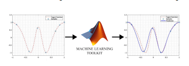
As stated previously, the acquisition process is traditionally done through fixed sampling schemes such as grid, random (RND), or Latin hypercube sampling (LHS), among various other approaches. In certain cases, these sampling schemes leave room for improvement by not taking into account aspects such as overall sampling density, output value swings or other information that can be extracted from the modeled circuit. This too, can be observed in the general example from Figure 1 in the area where points are not dense enough the predicted output differs more than in the regions which are sampled more densely. In this sense, adaptive sampling schemes [40] have advantages over fixed sampling schemes by sampling the input domain via an acquisition function 𝑎 𝑥 which takes into account aspects such as, model variance, sample density, or output swings. One such approach is sampling by model’s uncertainty/variance which was previously used with success for IC behavior modeling [1, 2, 3]. This way samples are selected based on the variation the model’s response in order to minimize the samples needed to develop a ML model. In order to obtain the best model for a given task, an intelligent approach must be taken. Consequently, an efficient sampling scheme can significantly benefit the overall model development process.
It has been shown previously in [1, 2, 3] that adaptive sampling methods based on active learning can offer a significant cost-benefit increase by incrementally sampling regions where the model error might improve significantly. The general method of sampling is highlighted in Figure 2. By developing an acquisition function based on the model’s uncertainty, we can overall improve overall model prediction, and hence, the overall fitting of the model. Previous research has shown the advantage of uncertainty-based sampling over fixed sampling methods both on synthetic functions and on IC use cases. The process of obtaining this uncertainty metric is discussed in further sections of this article.
The uncertainty sampling approach was preferred because it is computationally inexpensive. Any other adaptive sampling approach can be employed in the further presented sampling schemes.
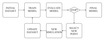
For the proposed uncertainty sampling scheme, the most appropriate ML algorithm is Gaussian process regression (GPR) [41] since it provides a mean prediction and a corresponding uncertainty function as outputs. The uncertainty output represents a 95% confidence interval of the mean prediction. This uncertainty output is used to improve the overall model behavior by sampling in the regions where its value is at a maximum.
A general example on a generic 1D function is given in Figure 3.
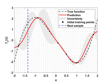
For this example, the best sample to improve model behavior is at the dashed blue line, since at that point the uncertainty of the prediction is at its highest. As a result, Figure 4 shows the new prediction with the added sample point included.
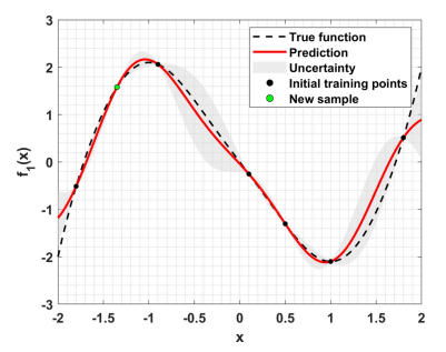
It is easily observable that in regions where points are not present or are sparse, the prediction differs from the target function, which is expected, and the uncertainty out-put of the GPR is significantly larger. Thus, by sampling in regions where this output is high improves the model. In some cases, GPR might be infeasible for several reasons. One of these reasons can be the high computational complexity of the algorithm, which for the GPR algorithm is 𝑂𝑁 3 . This can lead to high training times for large or high dimensional data sets.
3.1.1. Multiple output extension
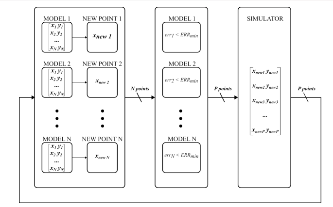
Since a single simulation run provides measurements for several outputs, the acquisition process naturally favors the development of multi-output sampling schemes. In this approach, all the outputs are modeled at the same time yielding from a speed-up in this case. The model development scheme presented in this article is based on an improved approach that has been used in prior research [3]. The improved sampling scheme is depicted in Figure 5.
The difference from the initial sampling approach is that for certain outputs the sampling will be stopped when they reach certain threshold errors imposed by the end user. This way a further simulation effort reduction is obtained by not oversampling some regions and at each iteration only 𝑃 samples are added, with 𝑃 𝑁 where
𝑁 is the number of outputs being modeled and 𝑃 is the number of outputs which are proposing a new point.
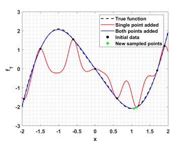
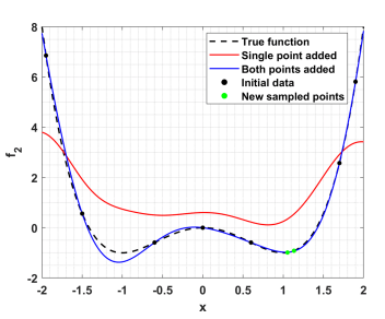
As a trivial example, we can take 2 general functions 𝑓1 and 𝑓2, defined as follows:
\[
f_1(x) = x^3 – 3\cdot x + 0.1\cdot \sin(1.5\pi x)
\tag{4}
\]
\[
f_2(x) = x^4 – 2\cdot x^2
\tag{5}
\]
The hypothesis is that 𝑓1 and 𝑓2 are dependent on each other and in a given application, the variation of 𝑥 either 1𝐷 or 𝑛𝐷 in a more general case can provide 𝑓1 and 𝑓2 at the same time. Given this aspect, each function will have an optimum sampling point which is depicted by the green point in both Figure 6 and Figure 7. Training each function only with its respective selected sampling points would result in the red-line function which would further
require more points, and the functions trained with both points, which have been acquired by one function evaluation each, would give us the blue-line function, which it is obviously more similar to the true function.
The diagram in Figure 5 can be further explained as follows. Let there be 𝑁 separate models, 𝑚 trained at iteration 𝑡 with their respective data sets 𝐷(𝑡), where 𝑛 ∈ {1…𝑁 }
\[
m_n(\mathbf{x}) \mid \mathcal{D}_n^{(t)}
=
\left\{(x_n,y_n)\right\}_{n=1}^{N}
\tag{6}
\]
Each model uses an acquisition function 𝛼𝑛 x (which relies on the model’s current uncertainty predictions) to propose exactly one new optimal candidate point:
\[
\mathbf{x}_{\mathrm{new},n}
=
\arg\max_{\mathbf{x}\in\mathcal{X}}
a_n\left(\mathbf{x};m^{(t)}\right)
\tag{7}
\]
This generates a set of 𝑁 candidate points:
\[
\mathcal{X}_{\mathrm{candidates}}
=
\left\{
\mathbf{x}_{\mathrm{new},1},
\mathbf{x}_{\mathrm{new},2},
\ldots,
\mathbf{x}_{\mathrm{new},N}
\right\}
\tag{8}
\]
We define a selection indicator function I𝑛 for each candidate point:
\[
I_n =
\begin{cases}
1, & \text{if } \operatorname{err}_n(\mathbf{x}_{\mathrm{new},n}) < \mathrm{ERR}_{\min} \\
0, & \text{otherwise}
\end{cases}
\tag{9}
\]
Applying this filter reduces the 𝑁 candidates down to a subset of 𝑃 points (𝑃 ≤ 𝑀):
\[
\mathcal{X}_{\mathrm{selected}}
=
\left\{
\mathbf{x}_{\mathrm{new},n}
\mid
I_n = 1
\right\}
=
\left\{
\mathbf{x}_{\mathrm{new},1},
\ldots,
\mathbf{x}_{\mathrm{new},P}
\right\}
\tag{10}
\]
Then the selected 𝑃 samples are simulated using the ground-truth simulator and obtain a new batch of training samples:
\[
\mathcal{D}_{\mathrm{batch}}
=
\left\{
\left(
\mathbf{x}_{\mathrm{new},p},
y_{\mathrm{new},p}
\right)
\right\}_{p=1}^{P}
\tag{11}
\]
Finally, the newly simulated data points are used to update the training sets for the next iteration 𝑡 ← 𝑡 + 1:
\[
\mathcal{D}_{n}^{(t+1)}
=
\mathcal{D}_{n}^{(t)}
\cup
\mathcal{D}_{\mathrm{batch}}
\qquad
\forall n
\tag{12}
\]
3.1.2. Testing machine learning models
For testing machine learning models different error metrics can be used. A set of popular error metrics are presented in Table 2 each of them having particular advantages.
In the experiments presented, results will be plot-ted using the relative RMSE (both in absolute value and percentage-wise) which takes into account also the output magnitude. The relative RMSE has an advantage over the other metrics because it takes into account the output swing by dividing the RMSE by the 𝐿2 norm. For a better evaluation several error metrics can be considered, such as using both the ME and relative RMSE as in [1, 2].
Table 2: Usual error functions used in ML testing.
| Function | Equation |
|---|---|
| Maximum error (ME) | \[ \mathrm{ME} = \max_{i} \left( y_i – m(x_i) \right) \] |
| Mean average error (MAE) | \[ \mathrm{MAE} = \frac{1}{n} \sum_{i=1}^{n} \left( y_i – m(x_i) \right) \] |
| Mean square error (MSE) | \[ \mathrm{MSE} = \frac{1}{n} \sum_{i=1}^{n} \left( y_i – m(x_i) \right)^2 \] |
| Root mean square error (RMSE) | \[ \mathrm{RMSE} = \sqrt{ \frac{1}{n} \sum_{i=1}^{n} \left( y_i – m(x_i) \right)^2 } \] |
| Relative RMSE | \[ \mathrm{RRMSE} = \frac{ \sqrt{ \frac{1}{n} \sum_{i=1}^{n} \left( y_i – m(x_i) \right)^2 } }{ \sqrt{ \sum_{i=1}^{n} y_i^2 } } \] |
| Relative RMSE [%] | \[ \mathrm{RRMSE}[\%] = \frac{ \sqrt{ \frac{1}{n} \sum_{i=1}^{n} \left( y_i – m(x_i) \right)^2 } }{ \sqrt{ \sum_{i=1}^{n} y_i^2 } } \times 100 \] |
Typically, the test set is a subset of the total available points, commonly between 10% and 20%. Given that we are trying to asses the validity of our sampling methods we took a larger testing set only for developmental purposes which will give us a more stable error over the number of samples added to the model. For the synthetic benchmark functions a set of 𝑛 = 200 points was used which covers the search space densely enough and for the ICs use cases a set of 𝑛 = 1000 points will be used. The test set will be and independent set which will not be used in the training of the ML models.
3.2. Optimization algorithms for integrated circuits
The optimization of analog ICs has the scope of maximizing or minimizing certain design specifications in a given search space. Literature proposes several frame-works in this sense, with various optimization algorithms having favorable results such as Bayesian optimization [19, 10, 11], Differential evolution [5, 6] or Genetic algorithms [20]. Further we will use Bayesian optimization with various objective function configurations given their popularity.
Bayesian optimization is one of the most accurate methods for determining a global optimum, the framework can outperform grid and random search but can be slow when many hyper parameters are involved [42].
The Bayesian optimization approach consists of t essential parts. The first part is the probabilistic surrogate model of the objective function, which is updated incrementally when new data is observed. With the probabilistic surrogate model, the model uncertainty can also be evaluated. The second part is an acquisition function, which is used to explore the state space based on the surrogate model optimally. The acquisition function aims to balance the exploration and exploitation during the optimization process. A typical acquisition function which is also the one we used in our experiments is the Expected Improvement (EI) function. A detailed guide and imple-mentation of Bayesian optimization can be found in [43] and [44].
The optimizer will aim to find the minimum of the unknown black-box function 𝑓 𝑥 defined by equation (13). The general mode of BO operation is presented in equation (14). The algorithm will aim to find the point 𝑥𝑚 which minimizes the response of 𝑓 (𝑥).
\[
f(x): X \rightarrow \mathbb{R}^{n},
\qquad
X \subseteq \mathbb{R}^{n}
\tag{13}
\]
\[
x_m
=
\operatorname*{arg\,min}_{x \in X}
f(x)
\tag{14}
\]
3.3. The overall proposed system
In Figure 8 we can observe the entire system depicted. Firstly, the model development which is done with MAT-LAB [45] and LTSpice [46] but other alternatives can be used as well. When the end user is satisfied with the over-all accuracy of the model or has reached the imposed simulation budget, the model can afterwards be used in the optimization process in order to size a predefined circuit topology to a set of design specifications. The advantage of this approach is that the model can be reused in several designs with different sets of specifications without further simulator use. Similarly, the bottleneck introduced by either the time needed to perform the simulations or the licensing costs attributed to the simulation environment becomes negligible.
In the presented results a BSIM3 model for the transistors was used in a standard 0.18𝜇𝑚 CMOS PDK. Nonetheless, the current approach allows for a easy technology
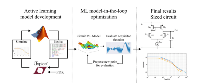
change, migration to another process can be done only by changing the PDK file.
For the optimization of hyperparameters the same BO framework can be employed. In the presented experiments Bayesian optimization with k-fold cross-validation was used. This is a powerful technique for hyperparameter tuning that balances efficiency and robustness. Bayesian optimization models the performance of hyperparameters as a probabilistic function and intelligently explores the search space to find the optimal settings. By incorporating k-fold cross-validation, the method ensures that performance estimates are reliable and not biased by a single train-test split. This combination allows for more in-formed decisions during the search process, leading to better generalization and model performance while reducing the number of evaluations needed compared to grid or random search.
As a kernel function the squared exponential function was used, which introduced two hyperparameters, namely, signal variance (𝜎2 ) and length scale (𝜎𝑙 ) according to equation (15)
\[
k(x,x’)
=
\sigma_f^{2}
\exp\left(
-\frac{(x-x’)^{2}}{2\sigma_l^{2}}
\right)
\tag{15}
\]
Additionally, the estimate of noise standard deviation (𝜎0) was considered as a hyperparameter in order to regulate over and under fitting of the model.
4. Experimental results
In this section, experimental results for the proposed approach are presented. Firstly, results on the proposed improved modeling approach will be presented on a set of synthetic functions which provides an easy way to test laborious algorithms and afterwards on the two mentioned IC use cases. The results are compared from the number of samples used to reach a certain error and also the error obtained in the imposed simulation budget.
Secondly, the developed models will be used in various optimization runs with BO and several optimization objectives in order to asses the utility of the proposed modeling technique.
4.1. Meta model development
4.1.1. Synthetic function results
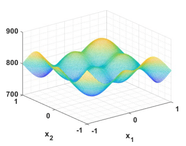
It is good practice to test complicated or time-consuming algorithms first on a set of low-dimension syn-thetic functions in order to assess the validity of the proposed algorithms. Below, we will highlight some preliminary results for a set of surrogate functions of 2D dimension (one graphical example being provided in Figure 9 and the rest in Table 3) which serve as a good baseline evaluation when designing new algorithms. These functions are in part popular benchmark functions found in literature [47] while a few are designed by hand.
Table 3: Equations for the functions used in the experiments.
| Name | Equation |
|---|---|
| F1 | \[ F_1 = \sum_{i=1}^{2} 50x_i \sin\left(\sqrt{|50x_i|}\right) \] |
| F2 | \[ F_2 = \sum_{i=1}^{2} 1000 \left( 1+ \exp\left(-\frac{2}{15}x_i^2\right) – 2\exp\left(-2x_i^2\right) \cos^2(2x_i) \right) \] |
| F3 | \[ F_3 = \prod_{i=1}^{2} \exp\left(-2x_i^2\right) \] |
| F4 | \[ F_4 = \prod_{i=1}^{2} \left[ 0.3 \exp\left( -\frac{ \left(x_i-0.5(-1)^i\right)^2 }{0.05} \right) + 0.6 \exp\left( -\frac{ \left(x_i-0.6(-1)^i\right)^2 }{0.05} \right) + \exp\left( -\frac{x_i^2}{0.05} \right) \right] \] |
| F5 | \[ F_5 = \sum_{i=1}^{2} \operatorname{sinc}(\pi x_i) \] |
| F6 | \[ F_6 = \sum_{i=1}^{2} \left[ \operatorname{sinc}(\pi x_i) + \tanh(\pi x_i) \right] \] |
| F7 | \[ F_7 = \sum_{i=1}^{2} \left[ x_i^2 + 0.5 \exp\left( -\frac{x_i^2}{0.2} \right) \right] \] |
| F8 | \[ F_8 = \sum_{i=1}^{2} \left[ |x_i^3| + \operatorname{sinc}(\pi x_i+1) \right] \] |
Every sampling method will be run for a total of 500 training samples, and averaged for a number of 10 runs to ensure an accurate interpretation of the errors. For the multi-output improved approach, the threshold for the models will be 0.001 which will mean a relative RMSE of 0.1%. This is realistic for the 2D functions given the complexity of the functions and the size of the testing set.
In practice, these thresholds cannot be known a priori because the exact performance landscape of a new circuit block is completely hidden prior to sampling, instead threshold selection is a direct reflection of the analog designer’s intuition balanced against their simulation budget. This will further be the case for our IC use cases as well.
From the results in Figure 10 and Tables 4 and 5 it can be observed that the ALS sampling for a single output performs the best, which is expected. Following that, we can see that on average, the ALS-MO sampling schemes (where ALS-MO is the standard parallel sampling approach and ALS-MO2 is the improved approach with the threshold implemented) yield results better than the fixed methods and slightly worse than the single-output sampling, which again is expected. Functions 𝐹3 and 𝐹4 are the simplest functions and hence are the easiest to model; for these functions, the differences between the methods are minimal.
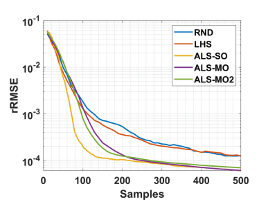
Table 4: Surrogate function – samples needed to reach 0.1 % error.
| Fun. | RND | LHS | ALS | SO | MO1 | MO2 |
|---|---|---|---|---|---|---|
| F1 | 104 | 99 | 70 | 90 | 84 | |
| F2 | 130 | 105 | 82 | 105 | 98 | |
| F3 | 140 | 120 | 80 | 120 | 120 | |
| F4 | 400 | 400 | 260 | 360 | 360 | |
| F5 | 320 | 260 | 100 | 160 | 140 | |
| F6 | 340 | 300 | 100 | 170 | 120 | |
| F7 | 130 | 120 | 90 | 110 | 100 | |
| F8 | 260 | 260 | 100 | 160 | 135 |
Table 5: Surrogate function – error at 300 samples.
| Fun. | RND | LHS | ALS | SO | MO1 | MO2 |
|---|---|---|---|---|---|---|
| F1 | 0.02% | 0.02% | 0.007% | 0.01% | 0.01% | |
| F2 | 0.02% | 0.02% | 0.009% | 0.009% | 0.009% | |
| F3 | 0.04% | 0.04% | 0.04% | 0.04% | 0.04% | |
| F4 | 0.2% | 0.16% | 0.007% | 0.18% | 0.18% | |
| F5 | 0.01% | 0.09% | 0.02% | 0.03% | 0.02% | |
| F6 | 0.1% | 0.1% | 0.003% | 0.03% | 0.04% | |
| F7 | 0.02% | 0.02% | 0.01% | 0.01% | 0.01% | |
| F8 | 0.1% | 0.08% | 0.04% | 0.04% | 0.04% |
The key takeaway from these results is that for functions that are modeled better (i.e., with lower error), there is no significant difference whether the respective model requests a new point or not, since it already provides an overall good representation of the function. Furthermore, channeling those points toward other functions offers a steeper descent in error relative to the number of samples, resulting in a better overall modeling of our functions.
4.1.2. Integrated circuit use cases
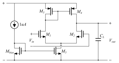
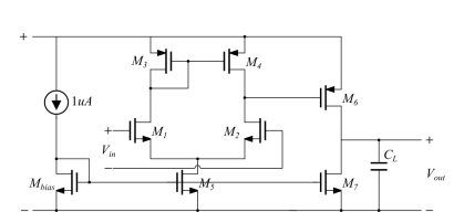
Based on the literature review from Table 1, two circuits were chosen as use cases, which are presented in Figure 11 and 12. In Figure 11 a single-stage operational amplifier is presented and in Figure 12 a two-stage operational amplifier which will serve as a more complex use case. The circuit in Figure 11 will have 6 input parameters to be modeled. They represent transistor lengths and width: namely,
𝑊1,2, 𝑊3,4 and 𝑊5 for the widths and 𝐿1,2, 𝐿3,4 and 𝐿5 for the lengths. The circuit in Figure 12 will have 4 more input parameters represented by the output stage parameters, 𝑊6, 𝐿6, 𝑊7 and 𝐿7. The other components present in the figures will be set at a fixed value in the presented experiments.
The input search domains for these use cases are as follows: the widths can vary between 10 𝜇m, 500 𝜇m and the lengths between 0.5 𝜇m, 5 𝜇m . More specific modeling tasks can employ different search spaces for each variable, as defined by the end user.
For these two use cases the outputs modeled will be a series of alternating current (AC) parameters, namely the AC Gain, common mode rejection ratio (CMRR) and power supply rejection ratio (PSRR). Given that these AC parameters are waveform dependent on the frequency of operation the values are averaged over several frequency intervals. The intervals as it can be observed in the Figure 13 are [1𝐻𝑧 − 10𝑘𝐻𝑧], [10𝑘𝐻𝑧 − 100𝑘𝐻𝑧], [100𝑘𝐻𝑧 − 1𝑀𝐻𝑧] and [1𝑀𝐻𝑧 − 10𝐺𝐻𝑧].
For the single stage OA the modeling budget will be 3000 points and for the two stage OA the budget will be raised to 5000 simulation points which are congruent with other papers propose as simulation budgets. As well as in the synthetic functions experiment the errors will be averaged over a number of 10 runs to have an accurate reading of the error gradient. For these use cases, only the fixed sampling methods implementation and the improved multi output sampling approach are presented. Furthermore, these ALS-MO models will be used in an BO optimization approach which will be presented in the following section.
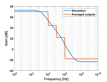
Figure 14 shows the error evolution across the number of samples. Table 6 and Table 7 contain the extracted data for all the modeled outputs. It can be observed that in this case some outputs not reach the desired 5% relative error but are relatively close. Sample-wise it can be concluded that a reduction of at least 33% was achieved for this threshold.
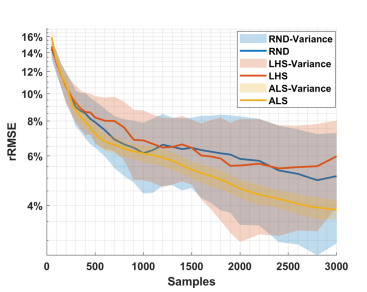
Table 6: Single stage OA – samples needed to reach 5 % error.
| Output | RND | LHS | ALS-MO |
|---|---|---|---|
| Gain1–10k | 230 | 220 | 180 |
| Gain10–100k | 2500 | – | 1500 |
| Gain100k–1M | – | 1800 | 980 |
| Gain1M–10G | 1200 | 1200 | 960 |
| CMRR1–10k | 1150 | 980 | 570 |
| CMRR10k–100k | 2950 | 2600 | 600 |
| CMRR100k–1M | 2300 | 2800 | 580 |
| CMRR1M–10G | 510 | 520 | 300 |
| PSRR1–10k | 100 | 100 | 100 |
| PSRR10k–100k | – | 2900 | 2000 |
| PSRR100k–1M | 1550 | 2200 | 1800 |
| PSRR1M–10G | 1300 | 1100 | 1150 |
Table 7: Single stage OA – error at 3000 samples.
| Output | RND | LHS | ALS-MO |
|---|---|---|---|
| Gain1–10k | 2.7% | 2.5% | 1.5% |
| Gain10–100k | 5% | 6% | 3.9% |
| Gain100k–1M | 5.5% | 4.8% | 3.9% |
| Gain1M–10G | 4.5% | 4% | 3% |
| CMRR1–10k | 4.7% | 4.5% | 3.4% |
| CMRR10k–100k | 4.6% | 4.7% | 3.4% |
| CMRR100k–1M | 4.6% | 4.4% | 2.8% |
| CMRR1M–10G | 3.2% | 3.4% | 2.5% |
| PSRR1–10k | 2.1% | 1.9% | 1.5% |
| PSRR10k–100k | 5.4% | 4.9% | 4.5% |
| PSRR100k–1M | 4.5% | 4.5% | 4.5% |
| PSRR1M–10G | 4% | 4% | 4% |
Figure 15 along with Table 8 and Table 9 presents the modeling process for the two-stage OA use case. Overall, the results are consistent with the synthetic function benchmark set and the single-stage OA. For this use case, a larger reduction in the required samples was achieved, representing at least a 48% reduction. Furthermore, it is important to note that for 𝐺𝑎𝑖𝑛1M 10G and all 𝐶𝑀𝑅𝑅 out-puts, the error in the fixed sampling case is significantly higher than in the adaptive case, further demonstrating the advantages of this approach.
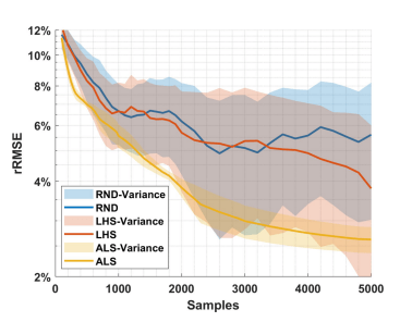
Table 8: Two stage OA – samples needed to reach 5 % error.
| Output | RND | LHS | ALS-MO |
|---|---|---|---|
| Gain1–10k | 2800 | 2800 | 2450 |
| Gain10–100k | 2600 | 3200 | 2300 |
| Gain100k–1M | 4500 | – | 2500 |
| Gain1M–10G | – | – | 800 |
| CMRR1–10k | 2550 | 3500 | 850 |
| CMRR10k–100k | 2100 | 2000 | 600 |
| CMRR100k–1M | 8500 | 1400 | 550 |
| CMRR1M–10G | 1900 | 1800 | 550 |
| PSRR1–10k | 2600 | 2600 | 2100 |
| PSRR10k–100k | 3800 | 2700 | 2600 |
| PSRR100k–1M | 4000 | 4200 | 2200 |
| PSRR1M–10G | 4500 | – | 2000 |
Table 9: Two stage OA – error at 5000 samples.
| Output | RND | LHS | ALS-MO |
|---|---|---|---|
| Gain1–10k | 4.5% | 4.5% | 4.5% |
| Gain10–100k | 4.5% | 4.5% | 4.5% |
| Gain100k–1M | 6% | 6.8% | 4.4% |
| Gain1M–10G | 7.5% | 7% | 0.4% |
| CMRR1–10k | 5% | 4% | 2% |
| CMRR10k–100k | 4.5% | 4.9% | 1% |
| CMRR100k–1M | 3% | 2.4% | 1.5% |
| CMRR1M–10G | 3.4% | 3.7% | 0.8% |
| PSRR1–10k | 4.3% | 3% | 2% |
| PSRR10k–100k | 5.2% | 4.7% | 5% |
| PSRR100k–1M | 5% | 5% | 4.5% |
| PSRR1M–10G | 4.5% | 4.9% | 4% |
4.2. Sensitivity analysis of the models
In this section, we aim to investigate certain aspects which are subject to variability, such as the predicted out-put regarding the number of averaged models, the variation in errors for all the modeled outputs, and the variability subject to the threshold errors of the outputs.
Firstly, the importance of segmenting will be investigated. Given that we are approximating a continuous waveform with a “discrete” approximation, in theory, a more compact interval sequencing would result in higher model fidelity regarding predictions. In practice, the segmentation of the frequency intervals is defined by the available computational power and, ultimately, by the experience of the analog designer.
Figure 16 highlights the results of several models trained with the same simulation data set but with different intervals used for averaging. It is clearly more reliable to divide the waveform into more models, using smaller frequency intervals, while keeping in mind the computational expense that comes with it. For more simple wave-forms, as it is shown in Figure 16 between pole-zero positions can be estimated with simple piece-wise approximations and difference between 2 successive intervals.
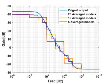
For this, the yellow trace in Figure 16 highlights clearly this since the models are averaged over each decade. For example, the two decades between 10𝑘𝐻𝑧 1𝑀𝐻𝑧 have a difference of 18𝑑𝐵 which correlates closely with a 20𝑑𝐵 decrease from the pole positioned around 1𝑘𝐻𝑧. Between 100𝑘𝐻𝑧 10𝑀𝐻𝑧 the difference drops to around 10𝑑𝐵 which is explained by the position of a zero which can be observed on the blue waveform, which represents the actual simulation.
Figure 17 and Figure 18 highlight the variation of modeling error for each output. These variations are computed from the means that are presented in Table 7 and Table 9 over the 10 previously mentioned runs. Equations (16 – 17) present the way in which these variations are computed:
\[
\tilde{E}
=
\frac{1}{N}
\sum_{i=1}^{N} E_i
\tag{16}
\]
\[
\mathrm{Variance}[\%]
=
\frac{
\frac{1}{N}
\sum_{i=1}^{N}
\left|E_i-\tilde{E}\right|
}{
\tilde{E}
}
\times 100
\tag{17}
\]
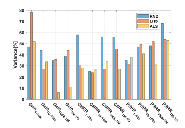
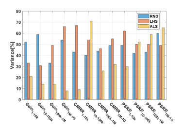
On average, for both use cases, the proposed adaptive sampling technique has a smaller variance of around 30% from the mean error, whereas their fixed sampling counterparts between 40 50% depending on the use case. Because this variation is relative to the mean error and not an absolute value, the resulting values are larger, but they highlight that the adaptive sampling method consistently yields better results.
Lastly, the influence of the threshold error on the size of the training data should be examined. To address this, a relation between the number of samples used in training and the testing error should be determined.
As an example, the single stage OA was selected, firstly the 𝐺𝑎𝑖𝑛100𝑘 1𝑀 dependency on the data size was modeled and afterward, all the model outputs were considered. Empirically, when training the models, the points at which certain key errors (15%, 10%, 5%, etc.) were reached and the number of samples required to reach those errors were collected in order to determine the dependency. A ML model was trained for this purpose, and a strong non-linear dependency can be observed from Figure 19.
Figure 20 the training data was obtained from all the modeled outputs to get a sense of general complexity of the circuit. In this example two distinct plateaus can be observed, one around the 7% and the other one around the 5% error threshold. This indicates that the training data size is beginning to yield diminishing returns.
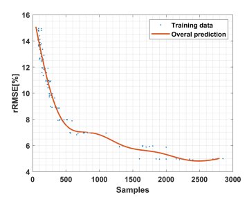
𝐺𝑎𝑖𝑛100𝑘−1𝑀 – single stage OA.
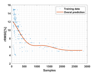
the outputs combined.
Naturally, the exact behavior of the error dependency remains highly circuit- or application-specific. However, a purely linear trend is highly unlikely, and an overall non linear relationship is expected nonetheless across most multi-output systems. This inherent non-linearity under-scores the necessity of a threshold-based sampling approach capable of capturing complex inter-dependencies without over-allocating simulation resources.
4.3. Meta model aided Bayesian optimization for IC sizing
The main scope of this article, is to investigate if there are any significant differences in using a ML-models-in-the-loop as a placeholder for actual simulation environments with regards to overall simulator use and the pro-posed solution. Even if the ML model approach does not use fewer evaluation points, the possibility of reuse in other tasks, such as redesign or verification, implies an advantage regarding the total use of the simulator.
As an acquisition function for the BO framework, the Expected Improvement (EI) function will be used, as it is one of the most popular functions. Also, since the BO framework returns the minimum of the function, all the objective functions will be negated in order to maximize the proposed objectives.
Since BO is a single objective optimizer, to optimize an IC that has multiple outputs to be maximized/minimized, a compounded function can be defined to assess the quality of the proposed design provided by the ML algorithm. This function is usually called a Figure of Merit (FoM) as well.
For the subsequent optimization runs, the models will utilize the 2000 training sample models for the single-stage operational amplifier and the 3000 training samples mod-els for the two-stage operational amplifier. These budgets assure a less than 5% error (or more than 95% accuracy) for most of the modeled outputs, as observed in Figure 14 and Figure 15.
4.3.1. Single stage operational amplifier use case
The first test was done on a single-objective optimization performed for the single-stage OA. For this test, the goal was to obtain a high DC gain; thus, only the first AC gain output of the modeled circuit was used.
In Figure 21 the results for the single objective optimization approach are presented. The iteration budget for the single stage amplifier was set to 200, similar to what other publications report. In Figure 22 we can we the simulation results for the circuits proposed by the BO run, and it can be observed there are no significant differences.
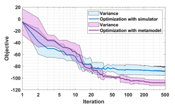
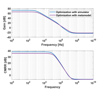
A more sophisticated approach is presented in the next figures. The proposed 𝐹𝑜𝑀1 expression is shown in equation (18). This approach aims to maximum equally the AC Gain and the CMRR up to 100 kHz. If desired, a weighted function can be designed in order to favor one output over the other by assigning different weights to the equation terms.
\[
FoM_1
=
\frac{
ACGain_{1\mathrm{Hz}-1\mathrm{kHz}}
+
ACGain_{10-100\mathrm{kHz}}
}{2}
–
\frac{
CMRR_{1\mathrm{Hz}-1\mathrm{kHz}}
+
CMRR_{10-100\mathrm{kHz}}
}{2}
\tag{18}
\]
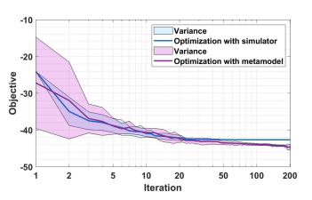
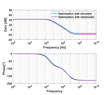
For the second run, we can observe a difference between the predicted objective with the ML model and the predicted objective with the simulator as shown in figure 23 and 24. This is mainly due to systematic error in the previously developed model, but it remains within tolerable margins.
stage operational amplifier.
4.3.2.Two stage operational amplifier use case
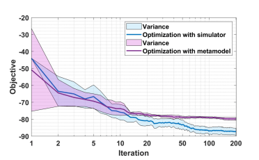
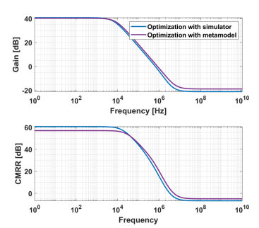
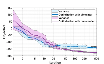
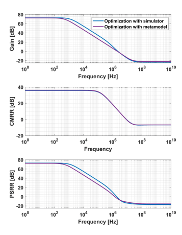
Further, we employed the same optimization objective from (18) for the second use case, which was the two-stage operational amplifier that has 10 input factors as shown in figure 25 and 26.
the two stage amplifier.
Lastly, we performed an optimization with all three outputs (AC Gain, CMRR and PSRR) as shown in figure 27 and 28, in the same format as previously shown and depicted in equation (19).
\[
FoM_2
=
–
\frac{
ACGain_{1\mathrm{Hz}-1\mathrm{kHz}}
+
ACGain_{10-100\mathrm{kHz}}
}{2}
–
\frac{
CMRR_{1\mathrm{Hz}-1\mathrm{kHz}}
+
CMRR_{10-100\mathrm{kHz}}
}{2}
–
\frac{
PSRR_{1\mathrm{Hz}-1\mathrm{kHz}}
+
PSRR_{10-100\mathrm{kHz}}
}{2}
\tag{19}
\]
of the two stage amplifier.
5. Conclusions
To conclude the article results, firstly the modeling approach will be discussed. An improvement to previous iterations of the proposed approach was done. By adding a threshold error to the modeled outputs and only taking into account points proposed by the models which are above the set threshold brings an improvement for the models which take more samples to model. The setting of the threshold can be either arbitrarily and adjusted during the sampling process if needed or either it can be set taking into account designer expertise and knowledge, the latter being the preferred approach.
A Bayesian optimization framework of analog integrated circuits was employed. The proposed approach used ML models in-the-loop instead of the actual simulation environment as an alternative aims to reduce heavy simulator use. The results which employed models with high accuracy (> 95%) had little to no significant difference in the end results between the two tested approaches. This might suggest that higher error models can be used (such as 10% relative RMSE) with a similar degree of success and should be further investigated.
In this article a much larger search space of the parameter design space is used than what is typically reported in literature, widths being varied between 10𝜇𝑚; 500𝜇𝑚 and the lengths between 0.5𝜇𝑚; 5𝜇𝑚 . This can easily help implement designs for a wider range of applications. Similar approaches used in literature usually set lower ranges for example up to 100 200𝜇𝑚 for the widths and up to 2𝜇𝑚 for the lengths of the transistors.
The central advantage of this approach is same model reuse for different tasks or different phases of the analog design cycle (such as design/optimization and pre-silicon verification afterwards) which are reported in literature. Also, given that the optimization algorithm can sometimes be entrapped in local optima, the ML model approach has a net advantage given that in theory an infinite number of evaluations can be done in the bounded search space.
The proposed approach can be easily migrated to other adaptive sampling strategies and integrated with several more advanced optimization frameworks, such as evolutionary algorithms or reinforcement learning, which might further improve the outcomes regarding circuit performance and overall model accuracy. The proposed frame-work aligns with standard industry design practices while offering both implementation simplicity and high computational efficiency. The primary advantage of this approach lies in the separation of the data acquisition phase from the optimization pipeline. Once the initial machine learning model is trained, the heavy computational burden of the analog simulator is entirely bypassed, allowing any chosen optimization algorithm to evaluate candidate designs instantly. This modularity makes the framework exceptionally useful in scenarios where multiple operational amplifier designs must be generated rapidly under varying constraints.
While a traditional simulation-backed Bayesian optimization (BO) loop requires launching a time-consuming SPICE simulation at every single iteration, the proposed model-in-the-loop framework evaluates candidate designs instantly via mathematical model. Consequently, subsequent optimization runs or adjustments to the design objectives (such as modifying the Figure of Merit weights) can be executed with virtually zero additional computational overhead. This shift from simulation-heavy to model-driven optimization fundamentally scales the efficiency of the design automation workflow, enabling rapid iterative redesign and verification without exhausting limited hardware simulator licenses.
As further research which might be of interest to explore how modeling behaves when different thresholds are set for the multi output approach and how it relates to the overall modeling. Further on how the overall models error relate to the ability to predict viable circuit sizing values. As mentioned in the previous paragraph higher error models could still be able to reach a robust circuit sizing.
- V. Grosu, E. David, L. Goras, G. Pelz, “Modelling integrated circuits behavior using an active learning approach based on gaussian process regression”, “2023 International Semiconductor Conference (CAS)”, pp. 245–248, 2023, doi:10.1109/CAS59036.2023.10303653.
- V. Grosu, L. Goras, E. David, G. Pelz, “Using neural network based active learning for modelling integrated circuits behavior”, “2023 International Symposium on Signals, Circuits and Systems (ISSCS)”, pp. 1–4, 2023, doi:10.1109/ISSCS58449.2023.10190907.
- V. Grosu, E. David, L. Goras, G. Pelz, “Multiple output modelling of integrated circuits behavior using an active learning approach”, “2024 20th International Conference on Synthesis, Modeling, Analysis and Simulation Methods and Applications to Circuit Design (SMACD)”, pp. 1–4, 2024, doi:10.1109/SMACD61181.2024.10745387.
- V. Grosu, E. David, L. Goras, G. Pelz, “On the modelling possibilities of integrated circuits behavior using active learning principles”, Romanian Journal on Information Science and Technology (ROMJIST), vol. 27, no. 2, pp. 183–195, 2024, doi:10.59277/ROMJIST.2024.2.05.
- C. Vişan, M. Sieberer, H. Cucu, “Designer-like automated circuit sizing for multiloop ldo”, “2023 International Semiconductor Conference (CAS)”, pp. 103–106, 2023, doi:10.1109/CAS59036.2023.10303725.
- C. Vişan, O. Pascu, M. Stănescu, E.-D. Şandru, C. Diaconu, A. Buzo, G. Pelz, H. Cucu, “Automated circuit sizing with multiobjective optimization based on differential evolution and bayesian inference”, Knowledge-Based Systems, vol. 258, p. 109987, 2022, doi:10.1016/j.knosys.2022.109987.
- A. Rusu, E. David, M.-D. Ţopa, V. Grosu, A. Buzo, G. Pelz, “On approaching multivariate ic pre-silicon verification using ml-based adaptive algorithms”, “2024 IEEE 30th International Symposium on On-Line Testing and Robust System Design (IOLTS)”, pp. 1–3, 2024, doi:10.1109/IOLTS60994.2024.10616057.
- A. Rusu, E. David, V. Grosu, M. Topa, A. Buzo, B. Carbunescu, G. Pelz, “On multivariate electrical performance machine learning driven pre-silicon ic adaptive verification”, IEEE Access, vol. 12, pp. 136436–136450, 2024, doi:10.1109/ACCESS.2024.3463393.
- D. Basso, L. Bortolussi, M. Videnovic-Misic, H. Habal, “Fast ml-driven analog circuit layout using reinforcement learning and steiner trees”, “2024 20th International Conference on Synthesis, Modeling, Analysis and Simulation Methods and Applications to Circuit Design (SMACD)”, pp. 1–4, 2024, doi:10.1109/SMACD61181.2024.10745442.
- P. P. Prajapati, M. V. Shah, “Automatic circuit design of cmos miller ota using cuckoo search algorithm”, International Journal of Applied Metaheuristic Computing (IJAMC), vol. 11, no. 1, pp. 36–44, 2020, doi:10.4018/IJAMC.2020010103.
- J. Huang, S. Zhang, C. Tao, F. Yang, C. Yan, D. Zhou, X. Zeng, “Bayesian optimization approach for analog circuit design using multi-task gaussian process”, “2021 IEEE International Symposium on Circuits and Systems (ISCAS)”, pp. 1–5, 2021, doi:10.1109/ISCAS51556.2021.9401205.
- M. Fukuda, T. Ishii, N. Takai, “Op-amp sizing by inference of element values using machine learning”, “2017 International Symposium on Intelligent Signal Processing and Communication Systems (ISPACS)”, pp. 622–627, 2017, doi:10.1109/ISPACS.2017.8266553.
- G. İslamoğlu, T. O. Çakici, E. Afacan, G. Dündar, “Artificial neural network assisted analog ic sizing tool”, “2019 16th International Conference on Synthesis, Modeling, Analysis and Simulation Methods and Applications to Circuit Design (SMACD)”, pp. 9–12, 2019, doi:10.1109/SMACD.2019.8795293.
- P.-O. Beaulieu, E. Dumesnil, F. Nabki, M. Boukadoum, “Analog rf circuit sizing by a cascade of shallow neural networks”, IEEE Transactions on Computer-Aided Design of Integrated Circuits and Systems, vol. 42, no. 12, pp. 4391–4401, 2023, doi:10.1109/TCAD.2023.3282570.
- N. Kahraman, T. Yildirim, “Technology independent automated sizing methodology based on artificial neural networks: An application to cmos opamp design”, “2014 International Conference on Computational Science and Computational Intelligence”, vol. 1, pp. 476–481, 2014, doi:10.1109/CSCI.2014.85.
- N. Lourenço, E. Afacan, R. Martins, F. Passos, A. Canelas, R. Póvoa, N. Horta, G. Dundar, “Using polynomial regression and artificial neural networks for reusable analog ic sizing”, “2019 16th International Conference on Synthesis, Modeling, Analysis and Simulation Methods and Applications to Circuit Design (SMACD)”, pp. 13–16, 2019, doi:10.1109/SMACD.2019.8795282.
- P. P. Prajapati, M. V. Shah, “Automated sizing methodology for cmos miller operational transconductance amplifier”, “Soft Computing: Theories and Applications. Advances in Intelligent Systems and Computing”, pp. 301–308, Springer, 2018, doi:10.1007/978-981-10-5699-4_29.
- W. Lyu, F. Yang, C. Yan, D. Zhou, X. Zeng, “Multi-objective bayesian optimization for analog/rf circuit synthesis”, “Proceedings of the 55th Annual Design Automation Conference”, DAC ’18, Association for Computing Machinery, New York, NY, USA, 2018, doi:10.1145/3195970.3196078.
- B. He, S. Zhang, F. Yang, C. Yan, D. Zhou, X. Zeng, “An efficient bayesian optimization approach for analog circuit synthesis via sparse gaussian process modeling”, “2020 Design, Automation & Test in Europe Conference & Exhibition (DATE)”, pp. 67–72, 2020, doi:10.23919/DATE48585.2020.9116366.
- A. Lberni, M. A. Marktani, A. Ahaitouf, A. Ahaitouf, “Analog circuit sizing based on evolutionary algorithms and deep learning”, Expert Systems with Applications, vol. 237, p. 121480, 2024, doi:10.1016/j.eswa.2023.121480.
- J. Gao, W. Cao, X. Zhang, “Rose: Robust analog circuit parameter optimization with sampling-efficient reinforcement learning”, “2023 60th ACM/IEEE Design Automation Conference (DAC)”, pp. 1–6, 2023, doi:10.1109/DAC56929.2023.10247991.
- Z. Li, A. C. Carusone, “Design and optimization of low-dropout voltage regulator using relational graph neural network and reinforcement learning in open-source sky130 process”, “2023 IEEE/ACM International Conference on Computer Aided Design (ICCAD)”, pp. 01–09, 2023, doi:10.1109/ICCAD57390.2023.10323720.
- Y. Li, Y. Wang, Y. Li, R. Zhou, Z. Lin, “An artificial neural network assisted optimization system for analog design space exploration”, IEEE Transactions on Computer-Aided Design of Integrated Circuits and Systems, vol. 39, no. 10, pp. 2640–2653, 2020, doi:10.1109/TCAD.2019.2961322.
- R. Mina, G. E. Sakr, H. Nassif, “Enhancing transistor sizing in analog ic design using a circuit-focused semi-supervised learning”, “2023 IEEE 4th International Multidisciplinary Conference on Engineering Technology (IMCET)”, pp. 223–228, 2023, doi:10.1109/IMCET59736.2023.10368264.
- Y. Uhlmann, T. Moldenhauer, J. Scheible, “Differentiable neural network surrogate models for gm/id-based analog ic sizing optimization”, “2023 ACM/IEEE 5th Workshop on Machine Learning for CAD (MLCAD)”, pp. 1–6, 2023, doi:10.1109/MLCAD58807.2023.10299834.
- Z. Zhao, L. Zhang, “Deep reinforcement learning for analog circuit sizing”, “2020 IEEE International Symposium on Circuits and Systems (ISCAS)”, pp. 1–5, 2020, doi:10.1109/ISCAS45731.2020.9181149.
- W. Lyu, F. Yang, C. Yan, D. Zhou, X. Zeng, “Batch Bayesian optimization via multi-objective acquisition ensemble for automated analog circuit design”, “Proceedings of the 35th International Conference on Machine Learning”, vol. 80 of Proceedings of Machine Learning Research, pp. 3306–3314, PMLR, 2018.
- N. Takai, M. Fukuda, “Prediction of element values of opamp for required specifications utilizing deep learning”, “2017 International Symposium on Electronics and Smart Devices (ISESD)”, pp. 300–303, 2017, doi:10.1109/ISESD.2017.8253353.
- A. C. Sanabria-Borbón, S. Soto-Aguilar, J. J. Estrada-López, D. Allaire, E. Sánchez-Sinencio, “Gaussian-process-based surrogate for optimization-aided and process-variations-aware analog circuit design”, Electronics, vol. 9, no. 4, 2020, doi:10.3390/electronics9040685.
- C. Vişan, M. Boldeanu, G. Nicolae, H. Cucu, C. Burileanu, A. Buzo, “Evolutionary bayesian optimization for automated circuit sizing”, Knowledge-Based Systems, vol. 318, p. 113483, 2025, doi:10.1016/j.knosys.2025.113483.
- F. Daylak, S. Ozoguz, “Automated neural networkbased optimization for enhancing dynamic range in active filter design”, Electronics, vol. 14, no. 4, 2025, doi:10.3390/electronics14040786.
- G. Huang, J. Hu, Y. He, J. Liu, M. Ma, Z. Shen, J. Wu, Y. Xu, H. Zhang, K. Zhong, et al., “Machine learning for electronic design automation: A survey”, ACM Transactions on Design Automation of Electronic Systems (TODAES), vol. 26, no. 5, pp. 1–46, 2021, doi:10.1145/3451179.
- D. V. Kochar, H. Wang, A. P. Chandrakasan, X. Zhang, “Ledro: Llm-enhanced design space reduction and optimization for analog circuits”, pp. 141–148, 2025, doi:10.1109/ICLAD65226.2025.00011.
- Y. Yin, Y. Wang, B. Xu, P. Li, “Ado-llm: Analog design bayesian optimization with in-context learning of large language models”, “Proceedings of the 43rd IEEE/ACM International Conference on Computer-Aided Design”, pp. 1–9, 2024, doi:10.1145/3676536.3676816.
- N. S. K. Somayaji, P. Li, “Llm-uso: Large language model-based universal sizing optimizer”, IEEE Transactions on Computer-Aided Design of Integrated Circuits and Systems, vol. 45, no. 4, pp. 1907–1920, 2026, doi:10.1109/TCAD.2025.3604643.
- C. Liu, E. A. Olowe, D. Chitnis, “Llm-based ai agent for sizing of analog and mixed signal circuit”, pp. 90–94, 2025, doi:10.1109/NewCAS64648.2025.11107079.
- C. Zhang, J. Jiang, Y. Zhao, “Euclidean space with orbital angular momentum”, “2019 IEEE International Conference on Communications Workshops (ICC Workshops)”, pp. 1–6, 2019, doi:10.1109/ICCW.2019.8756875.
- C. Zhang, J. Jiang, Y. Zhao, X. Jiang, “New degrees of freedom for beamforming manipulation in mimo transmission with oam”, “2019 IEEE Globecom Workshops (GC Wkshps)”, pp. 1–6, 2019, doi:10.1109/GCWkshps45667.2019.9024467.
- H. Niu, J. An, T. Wu, J. Chen, Y. Zhao, Y. Liang Guan, M. Di Renzo, M. Debbah, G. K. Karagiannidis, H. Vincent Poor, C. Yuen, “Introducing meta-fiber into stacked intelligent metasurfaces for mimo communications: A low-complexity design with only two layers”, IEEE Transactions on Wireless Communications, vol. 25, pp. 3016–3032, 2026, doi:10.1109/TWC.2025.3600915.
- J. N. Fuhg, A. Fau, U. Nackenhorst, “State-of-the-art and comparative review of adaptive sampling methods for kriging”, Archives of Computational Methods in Engineering, vol. 28, pp. 2689–2747, 2021, doi:10.1007/s11831-020-09474-6.
- C. K. Williams, C. E. Rasmussen, Gaussian processes for machine learning, Cambridge, MA: MIT press, 2006, doi:10.7551/mitpress/3206.001.0001.
- J. Bergstra, R. Bardenet, Y. Bengio, B. Kégl, “Algorithms for hyperparameter optimization”, vol. 24, pp. 2546–2554, 2011.
- B. Shahriari, K. Swersky, Z. Wang, R. P. Adams, N. de Freitas, “Taking the human out of the loop: A review of bayesian optimization”, Proceedings of the IEEE, vol. 104, no. 1, pp. 148–175, 2016, doi:10.1109/JPROC.2015.2494218.
- W. Lyu, P. Xue, F. Yang, C. Yan, Z. Hong, X. Zeng, D. Zhou, “An efficient bayesian optimization approach for automated optimization of analog circuits”, IEEE Transactions on Circuits and Systems I: Regular Papers, vol. 65, no. 6, pp. 1954–1967, 2018, doi:10.1109/TCSI.2017.2768826.
- MathWorks, “Matlab version: 9.13.0 (r2023b)”, 2023.
- LinearTechnology, “Ltspice (version 24.1)”, 2025.
- V. Plevris, G. Solorzano, “A collection of 30 multidimensional functions for global optimization benchmarking”, Data, vol. 7, no. 4, p. 46, 2022, doi:10.3390/data7040046.