Early Warning for Maritime Storm Formation Using Temporal Autoencoder-Based Anomaly Detection

(This article belongs to the Special Issue on SP9 (Special Issue on Multidisciplinary Sciences & Advanced Technology (SI-MSAT 2026)) and the Section Artificial Intelligence – Computer Science (AIC))
Export Citations
Cite
Srivastava, S. , Xu, H. , Yan, D. and Balasubramanian, R. (2026). Early Warning for Maritime Storm Formation Using Temporal Autoencoder-Based Anomaly Detection. Journal of Engineering Research and Sciences, 5(5), 19–39. https://doi.org/10.55708/js0505003
Snehashish Srivastava, Haiping Xu, Donghui Yan and Ramprasad Balasubramanian. "Early Warning for Maritime Storm Formation Using Temporal Autoencoder-Based Anomaly Detection." Journal of Engineering Research and Sciences 5, no. 5 (May 2026): 19–39. https://doi.org/10.55708/js0505003
S. Srivastava, H. Xu, D. Yan and R. Balasubramanian, "Early Warning for Maritime Storm Formation Using Temporal Autoencoder-Based Anomaly Detection," Journal of Engineering Research and Sciences, vol. 5, no. 5, pp. 19–39, May. 2026, doi: 10.55708/js0505003.
Storms remain a serious hazard at sea, exposing vessels to rapidly changing conditions that endanger human life and result in substantial economic losses. Satellite-based detection methods are widely used but require significant computational resources and depend on land-to-sea communication links, which may become unreliable during severe weather. Machine learning approaches offer strong potential for early detection; however, they typically rely on large labeled datasets that are often unavailable for rare or rapidly developing storms. Moreover, many existing models depend on predefined storm signatures, limiting their ability to adapt to previously unseen conditions in real time. To address these challenges, we propose a sensor-based framework for early detection of non-tropical maritime storms using key meteorological variables, including atmospheric pressure, humidity, wind speed, sea surface temperature, and near-surface air temperature. These variables can be measured directly by onboard sensors, enabling continuous monitoring without reliance on external communication infrastructure. The proposed method employs a temporal autoencoder trained exclusively on storm-free data to learn normal atmospheric patterns and detect anomalies associated with storm development. By identifying deviations from normal temporal behavior, the framework provides early warnings before storms fully develop. Comprehensive case studies using both synthetic and real-world meteorological data demonstrate that the proposed approach can detect developing storms in advance, achieving average lead times exceeding one hour while maintaining strong detection performance. These results highlight the potential of the framework as a practical and reliable solution for enhancing maritime safety.
1. Introduction
Storms and tropical cyclones remain among the most severe and unpredictable hazards faced by vessels at sea. Sudden changes in wind, rapid drops in atmospheric pressure, and rising wave height can occur within hours or even minutes, leaving crews with limited time to respond effectively. For vessels operating far from shore, such conditions can quickly become life-threatening. The Food and Agriculture Organization (FAO) estimates approximately 24,000 fishing-related fatalities worldwide each year [1]. Because many incidents involving unregistered and small-scale vessels are not formally reported, recent studies suggest that the actual number may exceed 100,000 annually [2]. These statistics highlight the continuing need for reliable and accessible storm monitoring and early-warning systems for maritime environments. Over the past several decades, advances in environmental sensing and numerical weather prediction (NWP) have significantly improved large-scale storm forecasting. Global observation systems (GOS) integrate data from satellites, ocean buoys, surface stations, and ship-based measurements to support weather prediction and marine hazard advisories [3]. National agencies such as the U.S. National Oceanic and Atmospheric Administration (NOAA) further combine satellite observations with drifting buoys, aircraft reconnaissance, and ship reports to track tropical cyclones and issue multi-day forecasts [4, 5]. Despite these advances, important limitations remain. Many maritime accidents still occur when vessels encounter rapidly evolving local weather conditions that are not detected or communicated in time [6]. Forecast uncertainty remains high in remote ocean regions where observational coverage is sparse and communication links may be unreliable.
Existing maritime weather monitoring systems often depend on satellite connectivity, shore-based processing, and subscription-based forecasting services [7]. These requirements can limit reliability, scalability, and accessibility for vessels operating far from shore or under constrained operational conditions. Small-scale fishing fleets are particularly vulnerable because they frequently lack continuous access to advanced communication infrastructure and real-time decision-support systems [2, 8]. In practice, vessels typically rely on voyage planning, broadcast weather forecasts, or direct onboard observation of changing environmental conditions such as falling pressure and shifting winds [4, 9]. Although these approaches are effective for large, well-forecast systems, they are often less reliable for short-lived, localized, or rapidly intensifying storms.
In this paper, we present an onboard framework for early storm detection using only standard meteorological sensors, including measurements of pressure, temperature, humidity, and wind. The proposed approach is based on an unsupervised autoencoder trained exclusively on historical fair-weather data for a specific region, enabling the model to learn normal atmospheric patterns and relationships among variables. During operation, the system continuously analyzes incoming sensor data and issues alerts when sustained deviations from these learned patterns are detected, indicating the early stages of storm development. Because the framework operates entirely onboard, it does not rely on external forecasts or internet connectivity. This design improves resilience to communication outages and makes the system practical for vessels operating under constrained onboard conditions.
The proposed framework addresses the continuing challenge posed by rapidly evolving local weather, even as large-scale cyclone forecasting improves. Earlier local warnings provide crews with valuable time to reef sail, adjust course, secure equipment, or seek shelter before conditions become hazardous. For vessel operators, especially small-scale fishers, the approach reduces costs by eliminating the need for subscription-based weather services or satellite data connections. These benefits extend beyond immediate onboard decision-making. For safety agencies and insurers, onboard anomaly logs provide objective, time-stamped records of deteriorating conditions, supporting accident investigations and fleet-level risk assessment. Importantly, the method is designed to be accessible to the fleets that need it most. Small-scale and artisanal fishers represent a substantial portion of the global maritime workforce and account for a significant share of casualties yet are often excluded from satellite-dependent solutions due to cost barriers. The main contributions of this paper are summarized as follows:
- We propose an onboard storm detection framework based solely on locally collected meteorological sensor data for real-time maritime early warning.
- The framework employs a temporal autoencoder trained on fair-weather observations to detect sustained deviations from normal atmospheric behavior associated with storm formation.
- The proposed approach targets short-lived and localized storms that may not be effectively captured by conventional broadcast forecasting systems.
- Comprehensive case studies using synthetic and real-world meteorological data demonstrate effective and reliable early-warning performance under realistic maritime operating conditions.
The rest of the paper is organized as follows. Section 2 reviews related work on deep learning-based storm analysis, anomaly detection, and autoencoder-based monitoring approaches. Section 3 presents the proposed storm detection framework. Section 4 describes the time-series data, feature selection process, and synthetic dataset construction. Section 5 discusses model training, hyperparameter tuning, and anomaly detection procedures. Section 6 presents threshold selection and evaluation metrics. Section 7 provides case studies and experimental results. Finally, Section 8 concludes the paper and discusses future research directions.
2. Related Work
Research on storm monitoring and early warning spans several interconnected areas, including deep learning-based weather analysis, anomaly detection in multivariate time series, and reconstruction-based learning methods such as autoencoders. This section reviews representative work in these areas and highlights how existing approaches differ from the storm formation detection framework proposed in this study.
2.1. Deep Learning-Based Storm Analysis
Weather forecasting has traditionally relied on physics-based NWP systems such as the Global Forecast System (GFS) and the Integrated Forecasting System (IFS) [10]. These systems simulate atmospheric behavior by solving the governing equations of atmospheric dynamics and thermodynamics while assimilating observations from satellites, buoys, radiosondes, and surface stations [11]. Although NWP models have improved substantially over recent decades, forecasting uncertainty remains relatively high over remote ocean regions due to sparse and irregular observations. This limitation affects the reliability of key variables such as sea-level pressure and wind speed, reducing forecasting accuracy in maritime environments far from measurement stations.
To complement physics-based forecasting, recent research has explored data-driven methods that learn relationships among atmospheric variables directly from historical observations. In tropical meteorology, machine learning and deep learning models have been used to predict tropical cyclone formation using satellite imagery and atmospheric reanalysis datasets. In [12], the authors evaluated random forests, support vector machines, and neural networks for predicting tropical cyclone formation with a 24-hour lead time. Similarly, in [13], the authors introduced a tropical cyclone formation dataset in which environmental variables are represented as multi-channel images centered on cyclone genesis locations. Many recent studies rely heavily on ERA5 reanalysis data [14], which provides globally consistent, high-resolution atmospheric variables for training and evaluating machine learning models. Deep learning methods have also shown promising results for convective storm prediction. In [15], a probabilistic deep learning framework using GOES-16 satellite observations and radar-derived event labels outperformed traditional logistic regression models, particularly by reducing false alarms. More recently, transformer-based architectures have been explored for modeling the life cycle of tropical cyclones using physically meaningful environmental variables such as wind velocity and vertical wind shear [16].
Despite these advances, most deep learning storm prediction systems depend on large labeled datasets derived from satellite imagery, radar products, or atmospheric reanalysis fields. These methods are generally designed for regional or basin-scale forecasting rather than continuous local monitoring of rapidly evolving storms. Maritime environments introduce additional challenges because observations are sparse and communication with shore-based systems may be intermittent. As a result, environmental conditions encountered during deployment may differ substantially from those represented in the training data, reducing reliability in operational settings. In addition, reliance on centralized processing and external communication infrastructure can introduce latency during severe weather events.
In contrast, the framework proposed in this study focuses on localized storm monitoring using only shipboard meteorological sensor data. Recent work has demonstrated the feasibility of onboard deep learning systems for maritime applications. For example, in [17], the authors proposed a self-adaptive framework that uses onboard and drone-based sensor data with Long Short-Term Memory (LSTM) models to forecast marine visibility in real time. Building on this direction, our work focuses on the early detection of storm formation using locally collected onboard observations.
2.2. Anomaly Detection in Multivariate Time Series
Anomaly detection has been widely studied across multiple domains where identifying abnormal patterns in data is critical for system monitoring, fault detection, and early warning systems [18]. Traditional approaches have been applied in areas such as industrial monitoring, network security, transportation systems, and supply chain management. In many of these settings, anomalies correspond to deviations from expected behavior that may indicate equipment failures, cyber intrusions, or unexpected operational events. In [19], the authors introduced the Tennessee Eastman Process as a benchmark for evaluating process control and fault detection methods. It simulates industrial operations, allowing researchers to develop and test monitoring and anomaly detection techniques under realistic conditions. In [20], the authors evaluated the effectiveness of several anomaly detection methods for intelligent transportation systems. Their study compares multiple algorithms across traffic datasets and highlights the importance of selecting appropriate detection techniques for complex real-world monitoring environments. In [21], the author proposed a supply chain anomaly detection approach that combines simulation with machine learning techniques to monitor disruptions in complex supply chain networks. The study shows that simulated operational scenarios can be used to train data-driven models to identify abnormal patterns and detect potential supply chain disruptions.
Recent advances in deep learning have significantly improved anomaly detection performance by enabling models to learn complex temporal and nonlinear relationships from large datasets [22]. Recurrent neural networks (RNNs), especially LSTM networks, have been widely used for anomaly detection in multivariate time-series data. In [23], the author proposed an LSTM-GAN model that combines LSTM networks with generative adversarial networks (GANs) to learn normal sequence patterns and identify abnormal behavior. In [24], an LSTM-based model was applied to anomaly detection in natural gas pipeline monitoring data using multivariate sensor measurements. More recent studies have introduced advanced architecture for time-series anomaly detection. DeepLog [25] uses LSTM networks to model system log sequences for anomaly detection in large-scale computing systems. OmniAnomaly [26] employs a stochastic RNN to capture complex temporal dependencies in multivariate time-series data. TranAD [27] adopts transformer-based architecture with attention mechanisms to model temporal dependencies and improve anomaly detection performance compared with existing baseline methods.
These studies demonstrate the effectiveness of deep learning methods for identifying abnormal patterns in complex sequential datasets. However, most existing anomaly detection research focuses on controlled systems such as data centers, manufacturing processes, or cloud infrastructure, where anomalies typically correspond to equipment faults, network intrusions, or operational failures. In contrast, storm development is a gradual environmental process characterized by coupled changes in multiple atmospheric variables. Detecting such events requires identifying sustained multivariate departures from normal meteorological behavior rather than isolated anomalies in engineered systems. The framework proposed in this study applies anomaly detection principles to maritime meteorological monitoring by identifying persistent deviations in atmospheric conditions that may indicate the emerging storm conditions. This approach is particularly suitable when labeled storm data are scarce and real-time monitoring relies solely on onboard sensors.
2.3. Autoencoder-Based Anomaly Detection
An autoencoder is a neural network that reconstructs its input through a compressed latent representation [28]. By learning normal patterns in the data, the model captures its underlying structure. This allows the network to encode the dominant relationships, and temporal characteristics present in normal observations. When new observations deviate from this structure, the reconstruction error increases, enabling anomaly detection without requiring labeled abnormal examples. As a result, autoencoder-based methods are widely used in sensor-driven monitoring applications. Several studies demonstrate the effectiveness of this approach in industrial and mechanical systems. For example, in [29], the authors applied an autoencoder to electrical current measurements from industrial motors and showed that reconstruction error can reliably distinguish between normal and faulty operating states. In [30], the authors proposed an autoencoder-based framework for monitoring rotating machinery using vibration signals. Their model learns normal machine behavior directly from raw sensor data and detects anomalies through reconstruction errors, avoiding the need for manually engineered features. More advanced architecture has also been investigated to enhance detection capability. In [31], the authors introduced an anomaly detection framework that combines dual autoencoders with GANs. By integrating reconstruction learning with adversarial training, their method achieves significantly improved detection performance in industrial inspection tasks.
Autoencoder architecture has also been extended to temporal sequence modeling, which is particularly important for multivariate time-series data with evolving sequential patterns. In [32], the author proposed an LSTM-based encoder-decoder model that learns normal temporal dynamics and identifies anomalies through reconstruction errors. Their results demonstrate that LSTM networks can capture long-term temporal dependencies and identify abnormal patterns in multivariate time-series data. Similarly, in [33], the authors developed an intrusion detection system for in-vehicle networks based on multiple LSTM autoencoder models. By analyzing features such as transmission intervals and payload variations, the system learns normal communication patterns in controller area network (CAN) traffic and identifies anomalous network behavior. In [34], the author introduced a recurrent autoencoder designed to learn compact representations of multivariate time series with missing data. Their model captures temporal dependencies within sequences and produces fixed-length representations suitable for tasks such as anomaly detection, classification, and time-series analysis.
Despite the success of autoencoder-based anomaly detection in many domains, its use in maritime meteorological monitoring remains limited. Most maritime anomaly detection studies focus on vessel trajectory analysis, navigation safety, or mechanical system monitoring rather than atmospheric observations [35]. However, modern vessels routinely collect meteorological measurements such as wind speed, atmospheric pressure, temperature, and humidity through onboard sensors, providing valuable information about changing conditions at sea. In this study, we apply autoencoder-based anomaly detection to real-time shipboard meteorological monitoring. The model is trained using fair-weather observations to learn normal relationships among atmospheric variables and detect sustained deviations that may indicate early storm formation. Because the framework operates entirely onboard using locally collected sensor data, it can provide continuous monitoring even in remote ocean regions.
3. A Framework for Detection of Storm Formation
The proposed framework employs an autoencoder trained on fair-weather meteorological data to enable real-time detection of storm formation using only onboard sensor measurements. Autoencoders are unsupervised neural networks that learn compact and informative representations of input data by encoding it into a lower-dimensional latent space and reconstructing it while minimizing reconstruction error [28]. When input patterns deviate from learned normal conditions, reconstruction error rises, providing an effective signal for detecting anomalous atmospheric behavior.
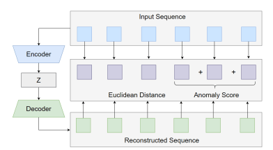
Figure 1 illustrates a standard autoencoder architecture consisting of three main components: an encoder (blue), a bottleneck layer (grey), and a decoder (green). The encoder maps a multivariate input sequence S into a low-dimensional latent representation z, while the bottleneck constrains the representation to capture only the most essential structure of the data. The decoder then reconstructs the original sequence from this latent representation z, producing output sequence S’.
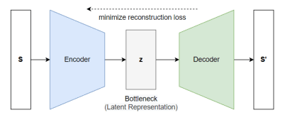
Formally, given an input sequence S, the encoder produces a latent representation z through a nonlinear function , as defined in Eq. (1).
\[
z = f_{\theta}(S)
\tag{1}
\]
The decoder subsequently reconstructs S’ from the latent vector z by applying another nonlinear function , as shown in Eq. (2).
\[
S’ = g_{\phi}(z)
\tag{2}
\]
By composing these two functions, the end-to-end autoencoder transformation is given in Eq. (3).
\[
S’ = g_{\phi}\!\left(f_{\theta}(S)\right)
\tag{3}
\]
The model is trained to minimize a reconstruction loss that measures the similarity between the input and reconstructed output. Let denote the feature vector at time step i, containing normalized readings of |F| meteorological variables. An input sample S is defined as a multivariate sequence of W consecutive feature vectors, as in Eq. (4).
\[
S = [x_{1}, x_{2}, \ldots, x_{W}] \in \mathbb{R}^{W \times |F|}
\tag{4}
\]
The reconstruction loss for a single sequence is defined as the mean squared error (MSE), averaged over the temporal dimension, as in Eq. (5).
\[
L(S,S’) = \frac{1}{W}\sum_{i=1}^{W} \left\| x_i – x_i’ \right\|^2
\tag{5}
\]
where \(x_{i,f}\) and \(x’_{i,f}\) represent the original and reconstructed feature vectors, respectively. The squared reconstruction error at time step i is computed across all features f F, as defined in Eq. (6).
\[
\left\| x_i – x_i’ \right\|^2
=
\sum_{f=1}^{|F|}
\left(x_{i,f} – x_{i,f}’\right)^2
\tag{6}
\]
where and are the observed and reconstructed values of feature f at time step i, respectively. Minimizing this loss allows the model to learn compact latent representations that preserve the dominant structure of fair-weather conditions. During real-time monitoring, sequences that deviate from these learned patterns produce higher reconstruction errors, indicating potential storm formation.
The encoder processes each multivariate sequence through temporal layers that may be convolutional, recurrent, or hybrid. Convolutional layers capture localized short-term variations, while recurrent layers model longer-term temporal dependencies. Nonlinear activation functions (e.g., tanh, ReLU, ELU) enable the network to represent complex relationships among variables, and dropout regularization is applied to improve generalization and reduce overfitting. At the center of the architecture, the bottleneck layer enforces a strong dimensionality reduction relative to the input size . This constraint prevents trivial memorization and encourages the model to retain only the most informative and recurring patterns associated with fair-weather. Consequently, the latent representation serves as a compact encoding of fair-weather conditions. The decoder mirrors the encoder structure and progressively reconstructs the original sequence from the latent representation. When the latent encoding accurately captures the underlying structure of the input, the reconstruction closely matches the original sequence. Conversely, unusual or previously unseen patterns result in degraded reconstruction quality, providing a measurable indicator of anomalous atmospheric conditions. In practice, training is performed using mini-batch optimization to improve computational efficiency and stability. Let be a batch of input sequences. The batch-level loss is defined as the average reconstruction loss across all sequences, as in Eq. (7).
\[
L(B,B’) = \frac{1}{b}\sum_{j=1}^{b} L(S_j,S_j’)
\tag{7}
\]
where b is the batch size, B’ denotes reconstructed outputs, and the model is trained through backpropagation to minimize this loss.
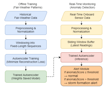
Figure 2 presents the overall framework, which consists of two main components: an offline training stage and a real-time monitoring stage. In the offline stage, historical fair-weather data are first preprocessed and segmented into fixed-length sequences using a sliding-window approach. These sequences are then used to train a temporal autoencoder to learn the characteristic patterns of normal marine conditions. Once training is complete, the learned model parameters are stored for operational deployment. In the real-time monitoring stage, incoming sensor readings undergo the same preprocessing procedure, and each updated sequence is provided to the trained autoencoder. The reconstruction error is evaluated by an alert module, which issues a warning when the error exceeds a predefined threshold. To reduce false alarms caused by noise or short-term fluctuations, the system emphasizes persistent and coordinated deviations across multiple variables rather than isolated spikes.
Overall, the proposed framework provides a robust and autonomous approach for early storm detection. By modeling normal atmospheric behavior through unsupervised learning, it enables continuous onboard monitoring without reliance on external satellite or radar data, supporting timely decision-making in diverse maritime environments.
4. Time-Series Data and Dataset Construction
4.1. Time-Series Data and Input Sequence
In our approach, the temporal autoencoder analyzes multivariate time series data to identify deviations from normal atmospheric patterns and provide early warnings before storms fully develop. The model input consists of meteorological variables arranged as fixed-interval sequences representing continuous temporal observations of evolving weather conditions. Because fair-weather conditions vary across geographic regions, each operational area exhibits its own baseline atmospheric behavior. A model trained in one region may interpret normal patterns in another as anomalies, leading to unreliable detections and false alerts. Therefore, each deployment region requires a localized model trained on fair-weather data representative of its specific meteorological and environmental conditions.
Each input sample is a multidimensional time series from the selected set of features F, recorded at fixed intervals (e.g., every 10 minutes), consistent with typical shipboard measurement frequencies. Since the variables are measured in different units, their raw magnitudes differ widely. For example, surface pressure can exceed 1,000 hPa, while humidity remains below 100%. Without normalization, features with larger numeric ranges could dominate the learning process. To prevent this imbalance, all variables are normalized to have a mean of 0 and a standard deviation of 1, which is done by subtracting the mean of all the readings of a feature from individual readings of that feature then dividing the result by the standard deviation of all the readings of the feature. Eq. (8) describes the normalization of each feature value \(x_{i,f}\) into its standardized form \(\hat{x}’_{i,f}\). Here, denotes the time index, \(f \in F\) represents a feature, and \(x_{i,f}\) is the observed value of feature f at time step i.
\[
\hat{x}_{i,f}
=
\frac{x_{i,f}-\mu(X_f)}
{\sigma(X_f)+\varepsilon}
\tag{8}
\]
The data normalization is performed using statistics computed from the historical dataset: Xf denotes the set of all historical observations of feature , from which the empirical mean \(\mu(X_f)\) and standard deviation \(\sigma(X_f)\) are calculated. A small constant is added to the denominator to prevent numerical instability when the standard deviation is close to zero. This standardization ensures that all features are centered at zero and scaled to comparable magnitudes prior to model training.
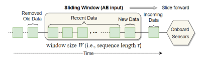
Figure 3 illustrates how the normalized time-series data are organized into overlapping sequences using a sliding-window mechanism. The same process is applied to both historical data during offline model training and incoming sensor measurements during real-time operation. A fixed-length window of size advances one time step at a time, continuously forming sequences that capture recent temporal evolution. At each step, the oldest data point is removed from the window, the newest observation is added, and the resulting sequence is passed to the autoencoder as input.
Formally, given a normalized multivariate time series \(\hat{D}\), as defined in Eq. (9), a sliding window is used to extract consecutive subsequences of length W.
\[
\hat{D} = \{x_1, x_2, \ldots, x_T\}
\tag{9}
\]
Here, each vector xt represents the readings of meteorological features at time step . Each sequence St of length is constructed as defined in Eq. (10).
\[
S_t = [x_t, x_{t+1}, \ldots, x_{t+W-1}]
\tag{10}
\]
The complete set of overlapping sequences is given by \(Win(\hat{D}, W)\), as defined in Eq. (11).
\[
Win(\hat{D}, W) = \{S_1, S_2, \ldots, S_{T-W+1}\}
\tag{11}
\]
This sequence construction ensures that consecutive sequences share most of their data, allowing the model to capture smooth temporal changes in atmospheric conditions. The window size determines how much historical context is available. Larger windows capture slower, large-scale trends but respond more slowly to sudden changes, while smaller windows are more sensitive to rapid developments but provide less long-term context. In this work, a window size of 15-time steps (150 minutes) provides an effective balance between sensitivity and temporal context, enabling the model to capture both short-term atmospheric fluctuations and the gradual evolution of pre-storm conditions. This sequence-based representation allows the model to learn temporal dependencies and evolving patterns rather than relying on isolated measurements.
4.2. Input Feature Selection
Reliable storm detection depends on selecting variables that reflect both stable fair-weather conditions and meaningful changes that precede storm onset. In this study, the chosen meteorological features were selected to represent the key physical and thermodynamic processes involved in storm development while remaining practical for real-world maritime deployment. A broader pool of candidate variables was first examined and evaluated according to their relevance to pre-storm dynamics and their suitability for short lead forecast time of 30 to 180 minutes. Variables that primarily represented post-storm effects, redundant information, or signals strongly influenced by non-atmospheric factors were excluded. Although many atmospheric parameters could be considered, the final feature set balances physical interpretability, predictive relevance, and availability from standard shipboard sensors. The model therefore incorporates five inputs: wind speed (WS), surface pressure (SP), 2-m air temperature (T2m), sea surface temperature (SST), and 2-m dew point temperature (D2m). Each variable has a well-established relationship with storm formation processes.
Wind speed (WS) is among the most responsive dynamic indicators. Convective storms frequently generate downbursts and gust fronts that produce sudden surface wind acceleration [36]. Rapid increases in wind speed often precede squalls and localized convective disturbances, making WS particularly informative for short-duration storm hazards. Wind speed is computed as shown in Eq. (12).
\[
WS = \sqrt{u_{10}^{2} + v_{10}^{2}}
\tag{12}
\]
where and represent the eastward and northward wind components at 10 m height. Together, these components describe the horizontal wind field, with negative values indicating westward or southward motion. Variations in surface wind speed are widely associated with the onset of both large-scale cyclones and localized storm cells.
Surface pressure (SP) provides another reliable early signal. Developing convective systems generate transient pressure perturbations and enhanced horizontal gradients near the surface. A drop in surface pressure has long been recognized as a precursor to tropical and extratropical storms [9]. Because pressure gradients drive low-level convergence and upward motion, surface pressure serves as a physically grounded and historically reliable indicator of storm intensification.
Near-surface air temperature, specifically the 2-m air temperature (T2m) influences atmospheric stability and buoyancy, both critical to convective initiation. Localized convective activity, including microbursts, may produce rapid surface cooling or warming depending on the dominant thermodynamic processes [36, 37]. Variations in T2m can indicate frontal boundaries, cold-pool formation, or destabilizing surface conditions that favor convection. Consequently, T2m provides meaningful insight into mesoscale storm evolution.
Sea surface temperature (SST) plays a fundamental role in storm energetics. By regulating surface heat and moisture fluxes, SST supports deep convection and influences near-surface temperature, pressure, and wind patterns [9, 38]. A threshold near 26.5 °C is often cited as necessary for storm development [9]. Including SST allows the model to account for the underlying oceanic energy source that fuels marine storms.
The 2-m dew point temperature (D2m) represents near-surface moisture availability. Unlike relative humidity, which depends on temperature and does not quantify moisture content, dew point reflects the actual amount of water vapor in the air. Higher D2m values indicate a moist boundary layer conducive to cloud formation and latent heat release, both of which promote convective growth [39]. Dew point is widely regarded as a key precursor variable in convective forecasting.
Additional variables were evaluated but ultimately excluded from the final model. For example, wave height generally increases in response to sustained wind forcing and therefore reflects storm conditions after intensification rather than during the early development stage [36]. Rainfall rate is typically observed once convection is underway and may be absent in dry downburst events. Relative humidity overlaps conceptually with dew point while also remaining strongly temperature dependent. Solar radiation largely follows diurnal variability and cloud fluctuations that are not uniquely tied to imminent storm formation. Reduced visibility is commonly associated with precipitation or fog that occurs after atmospheric cooling and saturation. Vessel roll and pitch were also excluded because ship motion is strongly influenced by vessel characteristics and operational factors, limiting their reliability as direct indicators of atmospheric conditions [40].
In summary, the five selected variables capture the essential thermodynamic and dynamic processes that precede or occur during storm formation. They provide complementary information without redundancy and can be measured using standard onboard instrumentation. By relying exclusively on locally observed sensor data, the framework avoids dependence on satellite imagery or external numerical weather model outputs. This design enables autonomous operation in remote marine environments where communication links may be limited, supporting practical storm formation detection at sea.
Evaluating early-warning performance using only real-world storm observations, however, remains challenging because storm onset times are often uncertain and environmental conditions can vary substantially across events. To enable systematic and controlled evaluation, we therefore constructed a high-resolution synthetic dataset that combines realistic fair-weather maritime conditions with simulated storm anomalies.
4.3. Construction of Synthetic Storm Datasets
The synthetic dataset was designed to generate controlled yet realistic storm development scenarios for evaluating detection accuracy and early-warning performance. In particular, it enables systematic analysis of lead-time performance under diverse pre-storm conditions. Unlike real-world datasets, where noise, missing observations, and irregular storm evolution can complicate evaluation, the synthetic environment provides controlled and reproducible conditions with clearly defined storm onset times.
Fair-weather sequences were generated using ERA5 reanalysis data [14] from equatorial and tropical maritime regions within the 10°–20° latitude belt. Periods without recorded storm activity, verified using the International Best Track Archive for Climate Stewardship (IBTrACS) archive [41], were selected. From these storm-free intervals, diurnal and seasonal patterns of selected meteorological variables, together with climatological trends, were extracted to construct a continuous six-month fair-weather period spanning January through June 2022. To preserve natural variability and emulate measurement uncertainty, Gaussian noise with standard deviations derived from real sensor observations was added to each variable. Additional constraints ensured physical realism, including enforcing valid value ranges and interpolating all variables to a 10-minute temporal resolution. While these sequences approximate real sensor dynamics, they provide a stable and interpretable baseline onto which synthetic storm events can be injected.
Synthetic storms were generated by introducing controlled, time-localized perturbations into the background data. Let xt denote the background feature vector at time. Modifications are applied only within the selected storm interval, leaving observations outside this interval unchanged. The injected signals are added directly to the background, producing a modified feature vector \(\tilde{x}_{t_i}\), as defined in Eq. (13).
\[
\tilde{x}_t = x_t + \Delta x_t
\tag{13}
\]
where \(\Delta x_{t_i}\) is nonzero only during the storm interval. This formulation ensures that storms remain embedded within realistic background variability rather than appearing as abrupt artificial spikes.
Each storm follows a three-phase temporal structure consisting of formation, maturity, and decay. The formation phase represents the pre-storm period during which environmental conditions gradually evolve toward storm-like behavior. The maturity phase corresponds to active storm conditions, and its onset, referred to as storm onset, is used to evaluate the early-warning performance of the proposed system. The decay phase models the gradual dissipation of the storm as meteorological variables return toward background levels.
Storm formation is governed by multiple physical interacting factors. Thermodynamic variables such as sea surface temperature, air temperature, and dew point influence whether a storm can develop but do not provide reliable markers for distinguishing transitions between formation, maturity, and decay. In contrast, wind speed and surface pressure exhibit clearer dynamical signatures during storm development. Storm intensification is associated with falling surface pressure that strengthens horizontal pressure gradients, which in turn accelerate wind speeds [11]. Accordingly, operational storm classification frameworks rely primarily on sustained wind thresholds, supported by pressure analysis [9].
Based on these principles, storm onset is defined using two criteria: (1) wind speed ≥ 11.3 m/s, consistent with the WMO lower bound for strong winds [9], and (2) surface pressure drop ≥ 3 hPa relative to the preceding 12-hour rolling mean. The pressure condition ensures that strong winds are associated with a developing low-pressure system rather than short-lived gusts. This dual criterion reflects the coupled relationship between pressure gradients and wind acceleration in developing storms [11]. While the maturity and decay phases share the same structure for comparability, the formation phase varies in duration and shape. This design enables simulation of diverse storm development scenarios and ensures that differences in detection performance arise primarily from variations in storm formation dynamics.
Figure 4 illustrates the wind speed evolution for a representative simulated storm event. The green curve represents fair-weather conditions, while the red curve shows simulated storm winds during the formation and maturity phases. The dashed horizontal line indicates the WMO strong-wind threshold of 11.3 m/s, and the vertical line marks storm onset.
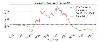
As shown in Figure 4, although wind speed exceeds this threshold during the formation phase, the storm is not declared immediately. Storm onset is defined only when wind speed exceeds the threshold and surface pressure drops at least 3 hPa below the preceding 12-hour rolling mean. Consequently, the initial threshold crossing occurs earlier than the declared storm onset, which appears later when the pressure condition is satisfied. This requirement prevents transient wind increases from being misinterpreted as storm formation and ensures that storm identification reflects the combined behavior of wind acceleration and pressure decrease during storm development. During the maturity phase, wind speed increases toward a peak and remains above the threshold. The decay phase then follows, producing a gradual return to background levels. Storm development is also accompanied by increased short-term wind variability. Under fair-weather conditions, fluctuations are relatively small, whereas during the storm both the mean wind speed and variability increase. To represent this behavior, the simulated storm signal amplifies local fluctuations during the storm interval, producing more irregular wind behavior during the maturity phase.
Figure 5 illustrates the evolution of surface pressure during a representative simulated storm event and the threshold-based method used to determine storm onset. The dashed gray curve represents the 12-hour rolling mean surface pressure, which serves as a reference for the background state. Green markers indicate fair-weather pressure values, while red markers represent values during the simulated storm period. The disturbance period begins when surface pressure falls below the rolling mean. However, storm onset is declared only when the pressure drops at least 3 hPa below this mean. The corresponding time is marked by the vertical gray line.
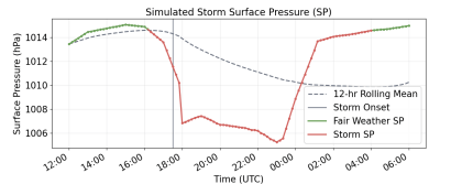
As shown in Figure 5, there is a short delay between the initial crossing and storm onset because the pressure must continue to decrease until the 3 hPa threshold is reached. In this example, this occurs after about two hours. Once the threshold is met, the system remains in the storm state while pressure stays below the background level. The storm ends when pressure gradually returns toward normal conditions and background atmospheric stability is restored. This definition avoids misinterpreting short-term fluctuations as storm formation and ensures that storms are identified based on sustained and physically meaningful pressure drops.
The simulation includes asynchronous changes across variables to better reflect real storm development. In the atmosphere, variables do not change at the same time. Surface pressure usually decreases first, which strengthens the pressure gradient and then increases wind speed. Thermodynamic variables such as temperature, sea surface temperature, and dew point may change earlier or later depending on local conditions. To model this, the simulation allows some variables to lead or lag slightly using small random time offsets during the formation phase. This avoids artificial synchronization while preserving physical relationships. As a result, the simulated storms show a more realistic pattern, where pressure drops, wind increases, and thermodynamic changes occur in sequence rather than all at once.
All storms reach similar intensity during the maturity phase and remain strong during this period. By keeping the maturity and decay phases consistent while allowing variation in the formation stage and across variables, the simulation produces storms that differ mainly in early development but remain comparable in peak intensity and duration. This design enables systematic evaluation of detection performance under diverse pre-storm conditions while maintaining a consistent definition of storm onset for lead-time analysis.
5. Autoencoder-Based Anomaly Detection
5.1. Autoencoder Training for Anomaly Detection
After initialization, the autoencoder is trained using overlapping time windows (i.e., fixed-length sequences) extracted from the background time series. Instead of updating the model with a single window at a time, multiple windows are grouped into mini-batches, and one update is performed per batch. The batch size plays an important role in both training stability and the model’s ability to capture normal variability. Very small batches can produce noisy and unstable updates, slowing convergence, while overly large batches may smooth the learned representation too much. This excessive smoothing can reduce sensitivity to subtle short-term changes that are important for early detection, potentially increasing false alarms or delaying detection.
To balance these effects, a moderate batch size is used to provide stable training while preserving natural variability. The batch size is selected empirically through systematic validation experiments by comparing training stability, reconstruction performance, and detection sensitivity across candidate values. This choice remains computationally efficient given the sequence length and number of input features, ensuring consistent and reproducible training. To further reduce potential overfitting, an early stopping strategy is applied. During training, reconstruction loss is continuously monitored on a separate validation set. If the validation loss does not improve for a predefined number of consecutive epochs (patience 𝑃), training is terminated and the model parameters corresponding to the lowest validation loss are retained as the final trained autoencoder. The overall training procedure is summarized in Algorithm 1.
| Algorithm 1: Autoencoder Training Procedure | |
|---|---|
| Input | Historical time-series dataset D, window size W, maximum epochs N, patience P |
| Output | Trained autoencoder M |
| 1 | D ← normalize(D) using Eq. (8) |
| 2 | Seq ← Win(D, W) using Eq. (11) |
| 3 | Split Seq into TrainSeq (first 80%) and ValSeq (last 20%) |
| 4 | Initialize autoencoder M with random weights |
| 5 | Set min_loss ← +∞; best_weights ← M.weights |
| 6 | Set no_improve ← 0 |
| 7 | Split TrainSeq into a set of mini-batches SMB |
| 8 | for epoch = 1 to N do |
| 9 | for each batch B in SMB do |
| 10 | B’ ← M(B) |
| 11 | ℒ ← L(B, B’) using Eq. (7) |
| 12 | Update M weights to minimize ℒ |
| 13 | Set val_loss ← 0 |
| 14 | for each sequence S in ValSeq do |
| 15 | S’ ← M(S) |
| 16 | val_loss ← val_loss + L(S, S’) using Eq. (5) |
| 17 | if val_loss < min_loss then |
| 18 | min_loss ← val_loss; best_weights ← M.weights |
| 19 | no_improve ← 0 |
| 20 | else |
| 21 | no_improve ← no_improve + 1 |
| 22 | if no_improve ≥ P then break |
| 23 | Load best_weights into M |
| 24 | return trained autoencoder M |
As shown in Algorithm 1, the input dataset is first normalized to obtain \(\hat{D}\) using the normalization scheme defined in Eq. (8). A sliding window operation is then applied to generate a list of overlapping sequences, denoted as , as defined in Eq. (11). The resulting sequences are divided into training and validation subsets, with the first 80% used for training ( and the remaining 20% reserved for validation . The autoencoder model is initialized with random weights, and the training sequences are grouped into mini batches. During each training epoch, the model reconstructs the input sequences and computes the average batch-level reconstruction loss using Eq. (7). Model parameters are then iteratively updated through backpropagation to minimize this loss. After all training batches in an epoch are processed, the model is evaluated on the validation set. The validation loss is computed by comparing the reconstructed sequences with the original validation data. If the validation loss improves over the best previously observed value min, the current model weights are saved and the early-stopping counter is reset; otherwise, the counter is incremented. Training terminates early if the validation loss does not improve for consecutive epochs. At termination, the model restores the weights corresponding to the lowest validation loss and returns the trained autoencoder .
5.2. Staged Grid Search and Architectural Design
Training a neural network involves adjusting its internal weights so that the model performs well with respect to a chosen objective function. For an autoencoder, this objective is to minimize reconstruction error, namely the difference between the original input and its reconstructed output. During training, the weights are updated iteratively using optimization algorithms such as stochastic gradient descent or Adam, gradually reducing reconstruction error on the training data. However, model performance is determined not only by the learned weights but also by a set of hyperparameters, including learning rate, activation function, dropout rate, batch size, hidden layer width, bottleneck dimension, and network depth. These choices strongly influence convergence speed, training stability, and generalization. Poorly selected hyperparameters can result in slow learning, unstable gradients, or overfitting.
In this study, we used a Gated Recurrent Unit (GRU)-based architecture to model storm formation dynamics within a 150-minute time window. Under normal conditions, atmospheric variables tend to change gradually rather than abruptly. Similarly, storm formation is typically preceded by a progressive buildup of instability, sustained moisture transport, and gradual near-surface atmospheric changes, instead of sudden isolated spikes. This means the modeling task mainly requires capturing short- to medium-range temporal dependencies rather than very long-term memory effects. GRUs are well suited for this purpose because their gating mechanisms allow the network to retain important information and discard irrelevant signals as the sequence progresses. This makes them effective at representing gradual temporal changes while using fewer parameters than other RNNs, such as LSTM models. The more compact structure also improves computational efficiency and often results in more stable training with lower risk of overfitting. By comparison, convolutional approaches such as Conv1D (1-Dimensional Convolutional Layer) are designed to capture localized temporal patterns using fixed receptive fields. While they are effective at identifying short motifs, they do not maintain an explicit hidden state that evolves over time. Since storm formation typically develops progressively, a recurrent architecture that tracks evolving temporal states provides a more natural way to represent atmospheric dynamics. Overall, the GRU-based architecture achieves a good balance between modeling capability and training efficiency for reconstruction-based anomaly detection in short- to medium-term forecasting.
To select appropriate hyperparameter values, we adopted a staged grid search strategy. In a standard grid search, all possible combinations within a predefined range are evaluated, and the configuration with the lowest validation error is selected. While this approach is systematic and reproducible, it can quickly become computationally expensive when many parameters are involved. For example, varying depth, layer width, and activation functions simultaneously leads to a rapid increase in the number of configurations, many of which are clearly suboptimal. To balance thoroughness and efficiency, we employed a staged search approach. Rather than tuning all hyperparameters simultaneously, we first determined the primary architectural settings and then progressively refined the remaining parameters. This staged strategy reduced computational cost while maintaining a transparent and systematic search process.
The hyperparameter tuning procedure consisted of three stages: architectural tuning, regularization tuning, and optimization tuning. The sequence was designed to first determine model capacity, then reduce overfitting, and finally refine training behavior. This approach allowed each group of parameters to be evaluated independently rather than adjusting all settings at once.
In the first stage, we focused on model depth and layer width, as these directly determine the model’s representational capacity. Model depth refers to the number of hidden layers in the encoder. Increasing depth allows the model to learn more abstract temporal patterns, but excessive depth may lead to instability or overfitting. Layer width represents the number of hidden units in each layer. Wider layers can capture richer temporal information, but they also increase the number of parameters and the risk of overfitting. We evaluated predefined depth and width combinations using validation reconstruction errors to identify architectures that provide sufficient capacity without unnecessary complexity. In the second stage, we tuned the activation function and dropout rate. The activation function affects gradient flow and convergence behavior, influencing how the model captures gradual versus sharp transitions in the data. Dropout serves as a regularization technique by randomly deactivating a portion of units during training, which reduces interdependence among neurons and improves generalization. These parameters were adjusted only after the architectural capacity had been fixed, ensuring a fair evaluation of their effects. In the final stage, we refined the optimization parameters, specifically the learning rate and batch size. The learning rate controls the magnitude of each weight update during training. If it is too large, training may become unstable; if too small, convergence can be slow or trapped in suboptimal solutions. Batch size determines how many samples are used to compute each gradient update. Smaller batches introduce more variability in the gradient, which can sometimes improve generalization but may reduce stability. Larger batches provide smoother updates and better computational efficiency. By tuning these parameters last, we were able to fine-tune the training dynamics after the architecture and regularization settings were established.
To ensure a fair comparison, all configurations were trained under identical experimental settings. The preprocessing steps, data splits, maximum number of epochs, and early stopping criteria were kept consistent across all experiments. Since the model was trained only on fair-weather data, validation reconstruction error was used as a consistent performance metric. To reduce the effect of random initialization, each experiment was repeated with multiple random seeds, and the results were averaged. At each stage of tuning, only the best-performing configurations were carried forward to the next stage. This progressive elimination approach helped reduce computational cost while keeping the search process structured and interpretable. The hyperparameter ranges were intentionally limited to maintain computational feasibility and analytical clarity.
Table 1 summarizes the grid search settings for the GRU-based autoencoder. The grid search experiments were conducted using ERA5 reanalysis data [14] extracted from tropical maritime regions within the 10°–20° latitude belt. Because atmospheric baseline conditions vary substantially across geographic regions, a four-month fair-weather segment preceding each storm case was selected. This design ensures that the learned fair-weather representation reflects the local geographic and climatological characteristics of the region in which the storm formed. ERA5 variables were obtained at hourly resolution and temporally interpolated to a 10-minute interval to match the sliding-window configuration. Applying a 150-minute sliding window with a 10-minute stride generated approximately 17,000 overlapping sequences. The sequences were divided chronologically to prevent temporal leakage, with the first 80% used for training and the remaining 20% reserved for validation. All models were trained with the Adam optimizer and mean squared error as the reconstruction loss. Early stopping with a patience of 15 epochs was employed to mitigate overfitting, and the model parameters corresponding to the lowest validation loss were retained.
Table 1: Grid search options for GRU-based autoencoders.
| Category | Options | Rationale |
|---|---|---|
| Model Depth | 1, 3, 5 | Evaluate increasing representational and hierarchical complexity. |
| Layer Width (Depth = 1) | 64, 128, 256 | Increase capacity with controlled parameter growth. |
| Layer Width (Depth = 3) | [64, 32, 16], [128, 64, 32], [256, 128, 64] | Enable stable and effective compression through gradual tapering toward the bottleneck. |
| Layer Width (Depth = 5) | [64, 32, 16, 8, 4], [128, 64, 32, 16, 8], [256, 128, 64, 32, 16] | Enable deeper hierarchical compression while maintaining controlled and balanced parameter growth. |
| Activation Function | ReLU, tanh, ELU | Affects gradient flow and convergence behavior. |
| Learning Rate | 5e−5, 1e−4, 2e−4 | Balance update magnitude with training stability and convergence. |
| Dropout Rate | 0.0, 0.2, 0.4 | Control regularization strength to mitigate overfitting. |
| Batch Size | 256, 512, 1024 | Balance gradient noise and training stability. |
In the first experiment, the width labels small, medium, and large correspond to specific hidden unit configurations at each depth, as defined in Table 1. For example, for depth 1, small, medium, and large represent 64, 128, and 256 units. Figure 6 presents the heatmap of validation loss across depth and width combinations. Increasing width generally reduces validation loss for depths 1 and 3, indicating that additional capacity improves reconstruction performance when the model depth is appropriate. Depth 3 consistently outperforms depth 1 across comparable width configurations, suggesting that three recurrent layers provide sufficient representational capacity for the temporal structure in the data. In contrast, depth 5 exhibits higher validation loss across all width settings, indicating excessive complexity and potential optimization difficulty. Because depth 3 with the large width configuration achieves the lowest validation loss, the architecture [256, 128, 64] is selected as the final configuration.
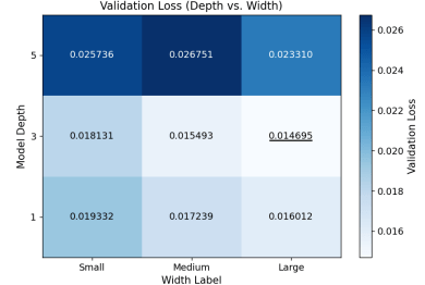
Figure 7 presents the heatmap of training and validation loss across activation functions and dropout rates. Each cell reports validation loss, with training loss shown in parentheses, and the color scale reflects validation loss. Dropout is evaluated by jointly examining both training and validation loss rather than relying on validation loss alone. A dropout rate of 0.0 yields the largest gap between training and validation loss, suggesting overfitting. A dropout rate of 0.4 reduces this gap but increases both losses, indicating underfitting. A dropout rate of 0.2 provides the best balance, maintaining low validation loss with a small generalization gap. Among the activation functions, ReLU consistently achieves the lowest validation loss. Therefore, ReLU with a dropout rate of 0.2 is selected for the next stage.
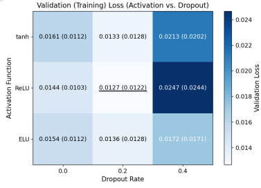
Figure 8 shows validation loss across learning rates and batch sizes for the selected architecture, with depth, width, activation function, and dropout fixed. Smaller batch sizes introduce greater gradient variability, which may improve generalization, while larger batches produce smoother updates and improved computational efficiency. The learning rate controls the magnitude of parameter updates during training. Excessively large values may cause instability, whereas very small values slow convergence. A learning rate of 2e-4 consistently yields the lowest validation loss across batch sizes. A batch size of 256 achieves the best overall performance, particularly at 2e-4, while performance degrades as batch size increases. This suggests that excessively large batches reduce beneficial gradient variability. A batch size of 256 corresponds to approximately 42 hours of sequential data per update, providing a balanced gradient estimate. Accordingly, a learning rate of 2e-4 with a batch size of 256 is selected for subsequent experiments.
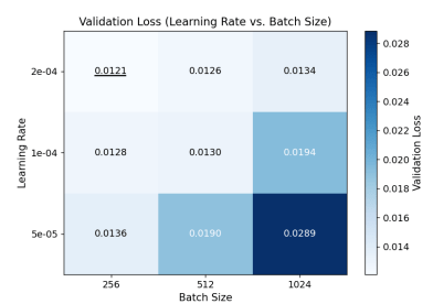
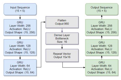
Figure 9 illustrates the final GRU-based autoencoder with ReLU activation, three recurrent layers, and a bottleneck dimension of 16. The model follows a sequence-to-sequence design: Input → GRU encoder stack → bottleneck → RepeatVector → GRU decoder stack → reconstructed sequence. Blue shaded layers denote the encoder, green shaded layers denote the decoder, and the gray shaded region indicates the bottleneck. The layer sizes follow the configuration [256, 128, 64].
The methodological choices in this study were guided by the operational requirements of maritime storm monitoring and the characteristics of the available data. The proposed framework emphasizes modeling evolving atmospheric conditions using only onboard sensor measurements, without reliance on satellite imagery or large labeled storm datasets. Compared with more complex architectures such as transformer-based models, the GRU-based autoencoder provides a favorable balance among temporal modeling capability, computational efficiency, and training stability for short- to medium-term sequence reconstruction. The selected features and sequence window were chosen to capture meaningful pre-storm atmospheric behavior while reducing redundancy and sensitivity to short-term noise. In addition, the staged grid-search procedure ensures that architectural and optimization settings are determined systematically through controlled validation experiments rather than ad hoc empirical selection.
5.3. Real-Time Anomaly Detection for Storm Formation
The real-time anomaly detection module operates continuously as the vessel moves, processing incoming sensor measurements to monitor evolving weather conditions. It maintains a sliding window containing the most recent observations, where each observation includes meteorological features. At each time step , the window is updated with the latest measurement. The resulting sequence is normalized using the mean and standard deviation computed from the historical training dataset, as defined in Eq. (8), and then passed through the trained autoencoder to generate a reconstruction. Let the normalized input sequence be represented by matrix S, as defined in Eq. (4). To quantify reconstruction accuracy, an error score is computed for each time step by measuring the Euclidean distance between the input and reconstructed feature vectors. For each , the reconstruction error ej represents the difference between the input feature vector xj and the reconstructed feature vector xj, as defined in Eq. (14).
\[
e_j
=
\sqrt{\left\|x_j – x_j’\right\|^2}
=
\sqrt{\sum_{f \in F}
\left(x_{j,f} – x_{j,f}’\right)^2}
\tag{14}
\]
where x_{j,f} is the value of feature f F at time step j, and xj is the vector of all feature values at time step j. This yields an error sequence (S, S’), as defined in Eq. (15).
\[
\mathrm{Error}(S,S’) = [e_1, e_2, \ldots, e_W]
\tag{15}
\]
which reflects the reconstruction accuracy at each time step in the input sequence. To emphasize recent behavior, an anomaly score at time t, denoted At, is computed as the sum of reconstruction errors over the most recent time steps, as defined in Eq. (16).
\[
A_t = \sum_{q=0}^{n-1} e_{t-q}
\tag{16}
\]
Figure 10 illustrates how the anomaly score is calculated. The input sequence is first reconstructed by the autoencoder, and the Euclidean distance between the original and reconstructed sequences is computed at each time step. The anomaly score is then obtained by aggregating reconstruction errors over a short temporal window (e.g., the latest three time steps), providing a real-time measure of deviation from learned normal behavior.
During storm development, using the entire input sequence may delay detection because earlier fair-weather data can hide emerging changes, while relying on a single data point may cause false alarms due to small fluctuations. As shown in Figure 10, to balance sensitivity and timeliness, the anomaly score is computed using three recent data points, corresponding to the most recent 30 minutes. Although the score is calculated from this short window, the autoencoder reconstructs a longer input sequence, so recent outputs are influenced by earlier observations. This allows gradual changes that start earlier to affect later reconstructions, improving detection of slowly developing anomalies. The resulting anomaly score reflects At how current observations differ from learned fair-weather patterns rather than indicating storm intensity. To further reduce false alarms, a persistence-based strategy is applied. When the anomaly score first exceeds a predefined threshold, the system issues an advisory alert. If the exceedance persists and At+1 remains above the threshold across consecutive windows, the condition is classified as sustained, and the alert is escalated to a critical level. This two-stage mechanism improves stability while maintaining timely detection of significant and persistent anomalies.
Algorithm 2 summarizes the overall real-time storm detection procedure, describing how incoming sensor measurements are processed, how reconstruction errors are evaluated, and how anomaly scores are used to trigger alerts. As outlined in the algorithm, the process combines reconstruction-based anomaly scoring with a persistence-aware alerting strategy. Rather than reacting to isolated threshold exceedances, the algorithm monitors whether anomalous behavior persists over consecutive time steps. This approach helps distinguish meaningful storm-related deviations from short-lived environmental fluctuations, reducing false alarms while allowing timely escalation when abnormal conditions are sustained. Consequently, the framework is well suited for real-time storm monitoring in dynamic marine environments.
Algorithm 2: Real-Time Detection of Storm Formation
Input: trained autoencoder model M, window size W, anomaly threshold θ, incoming sensor readings for features F, span n with 1 ≤ n ≤ W
Output: advisory and/or critical alerts
- Initialize input sequence S of shape W × |F|.
- Set
Alert_counter← 0. - While sensor readings continue do
- Update input sequence S with most recent W data.
- Normalize S using Eq. (8).
- Compute reconstruction sequence S’ ← M(S).
- Compute the error sequence Error(S, S’) using Eq. (15).
- Compute the anomaly score At using Eq. (16).
- If At > θ then
- If
Alert_counter≥ n then - Emit critical alert.
- Else
- Emit advisory alert.
Alert_counter←Alert_counter+ 1.- Else
Alert_counter← 0.
6. Threshold Selection and Evaluation Metrics
The anomaly detection thresholds used in this study are derived from the statistical characteristics of anomaly scores during fair-weather conditions. Because the autoencoder is trained exclusively on normal atmospheric data, the reconstruction error during these periods reflects the expected background variability of the system. Deviations from this baseline therefore indicate unusual atmospheric behavior that may be associated with storm development. Consequently, the anomaly score distribution under fair-weather conditions provides a natural reference for defining detection thresholds. To determine an appropriate threshold, anomaly scores were computed from fair-weather observations. Restricting the analysis to fair-weather data ensures that thresholds are defined independently of storm events. The mean (\mu) and standard deviation (\sigma) of the fair-weather anomaly scores were calculated to characterize baseline variability. Detection thresholds were then defined using the mean-standard deviation formulation, specifically \mu + \sigma,\ \mu + 2\sigma,\ \text{and}\ \mu + 3\sigma, , and , to capture different levels of sensitivity. This approach provides a statistically grounded method for distinguishing typical variability from progressively rarer deviations. Because storm formation represents a rare departure from normal atmospheric behavior, thresholds based on multiples of the standard deviation provide a simple and interpretable way to identify statistically significant deviations from the learned baseline. In statistical terms, these thresholds correspond to increasingly high percentile of the fair-weather anomaly score distribution. If the reconstruction errors are approximately normally distributed \mu + \sigma, corresponds to roughly the upper 84.1st percentile, meaning that about 15.9% of fair-weather observations may exceed this value. The \mu + 2\sigma threshold corresponds to approximately the 97.7th percentile, capturing only the most unusual deviations, while \mu + 3\sigma represents an extreme boundary near the 99.87th percentile, where only very rare anomalies are expected to occur under fair conditions. As the threshold increases, the detection mechanism becomes stricter, since only larger deviations from the learned normal pattern are classified as anomalous.
For evaluation, we consider a 12-hour observation window prior to each storm event, while a 180-minute detection window represents the operational warning horizon before storm onset. The 180-minute interval was selected because storm predictions made significantly earlier than three hours before storm onset may become less reliable due to the highly dynamic and localized nature of rapidly developing maritime storms. A three-hour warning horizon therefore provides a practical balance between early warning capability and prediction reliability while still allowing sufficient time for operational response and safety preparation. To assess the operational usefulness of the proposed system, lead time is used as a primary performance metric. Lead time measures how early the system can issue a reliable warning before storm onset. Within this detection window, the first critical alert is used to compute lead time. Specifically, lead time is defined as the interval between the first critical alert, issued at time t, and the observed storm onset at time ta, as given in Eq. (17).
\[
L = \max(t_s – t_a,\, 0),
\qquad
t_a \leq (t_s – 180)
\tag{17}
\]
The first critical alert at time constitutes a valid detection point only if it occurs within the 180-minute detection window prior to storm onset. If the first critical alert is issued after storm onset, the lead time is set to zero. Only critical alerts are considered in this calculation. Advisory alerts represent preliminary warning stages and may indicate increasing anomaly levels; however, they are insufficient to trigger an operational storm declaration. By focusing on critical alerts, the lead time reflects actionable warnings rather than intermediate signals. In the context of storm formation detection, lead time directly reflects the practical value of the system. A warning issued only moments before storm onset provides limited opportunity for preparation, mitigation, or safety measures. Conversely, artificially increasing lead time, typically by lowering the detection threshold, can substantially increase false alarms. In such cases, minor or transient anomalies may be incorrectly flagged as storm precursors. Therefore, lead time must be interpreted alongside precision and false alarm behavior. A large lead time is meaningful only if it is achieved without excessive false detections.
At each time step in a 12-hour window prior to a storm event, the model output can be either a prediction of fair weather (i.e., no alert) or an alert. The time-step categories used for precision evaluation are defined as follows.
- True Positive (TP): An alert issued within the 180-minute detection window before storm onset.
- False Positive (FP): An alert issued earlier than 180 minutes before storm onset, within the 12-hour observation window.
- True Negative (TN): A no-alert prediction issued during the 12-hour observation window but prior to the first critical alert within the 180-minute window.
- False Negative (FN): A no-alert prediction issued within the 180-minute detection window after the first critical alert has been issued.
Because the goal of the system is to provide operationally relevant short-term warnings for rapidly developing non-tropical storms, alerts issued more than 180 minutes before storm onset are treated as false positives for evaluation purposes. After the first critical alert is issued, subsequent no-alert predictions may occur because of sensor noise, missing data, or model limitations. Such outputs are counted as false negatives, since the correct system behavior at that stage is to continue issuing alerts until storm onset. Table 2 summarizes the time-step classification scheme used for precision evaluation within the 12-hour observation window, including the 180-minute detection window.
Table 2: Time-step classification scheme used for precision evaluation.
| Model Output | Time Relative to Storm Onset | Classification |
|---|---|---|
| Alert | Within 180 minutes before storm onset | TP |
| Alert | Earlier than 180 minutes before storm onset, within the 12-hour window | FP |
| No Alert | During the 12-hour window and before the first critical alert in the 180-minute detection window | TN |
| No Alert | Within the 180-minute detection window, after the first critical alert has been issued | FN |
Because storm events are rare relative to fair-weather conditions, the dataset is highly imbalanced. Most time steps correspond to normal conditions, while storm onsets occur only occasionally. In such cases, overall accuracy can be misleading. For example, if storms occur in only 5% of the timeline, a model that always predicts “no storm” would still achieve 95% accuracy, despite failing to detect storms. Therefore, accuracy alone does not provide a meaningful measure of performance for rare-event detection. To better evaluate detection quality, we rely on metrics derived from the confusion matrix. Precision, recall, and F1 score are defined in Eqs. (18–20).
\[
\mathrm{Precision}
=
\frac{TP}{TP + FP}
\tag{18}
\]
\[
\mathrm{Recall}
=
\frac{TP}{TP + FN}
\tag{19}
\]
\[
F1
=
2 \cdot
\frac{\mathrm{Precision} \cdot \mathrm{Recall}}
{\mathrm{Precision} + \mathrm{Recall}}
\tag{20}
\]
Precision measures how often issued alerts are correct. High precision means that when the system raises an alert, it likely corresponds to an actual storm. This is important in practice, since frequent false alarms can reduce user trust and lead to alarm fatigue. Recall measures how many storm formation events are successfully detected. High recall ensures that events are not missed, which is critical for safety and timely response. The F1 score combines precision and recall into a single measure using their harmonic mean. Unlike accuracy, it focuses on the positive (storm) class and balances two competing goals: detecting as many storm formation events as possible (high recall) while minimizing false alarms (high precision). Because the harmonic mean penalizes large imbalances between precision and recall, a high F1 score is achieved only when both are reasonably strong. For rare-event problems such as storm formation detection, the F1 score provides a more informative and operationally meaningful measure than overall accuracy. It reflects the system’s ability to detect storms reliably without generating excessive false alarms, which is essential for practical deployment.
Figure 11 illustrates representative examples of TP, TN, FP, and FN within the proposed storm formation alerting framework. In Figure 11, advisory alerts (yellow), critical alerts (red), and normal conditions (green) are determined relative to the anomaly detection threshold (red dashed line). The red dashed horizontal line represents the anomaly detection threshold, while the vertical blue line marks the observed storm onset. A circle (O) denotes a correct classification, corresponding to either a TP or TN, whereas a cross (X) indicates an incorrect classification, representing either a FP or a FN.
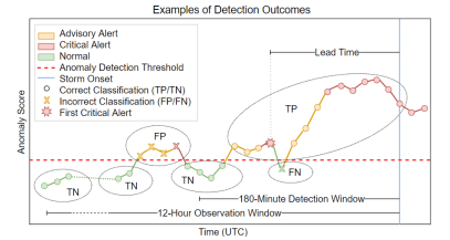
The red eight-point star in Figure 11 indicates the first critical alert used to compute the lead time. According to the detection rule, the first critical alert occurring within 180 minutes prior to storm onset is considered the valid detection point. Once this alert is issued, any subsequent time step within this interval classified as normal weather is counted as a false negative (FN), since the system has already identified the developing storm condition.
7. Case Studies
To evaluate the usefulness of the proposed sensor-based autoencoder framework for early storm detection, we conducted a case study using both synthetic data and real meteorological observations. The framework was first tested in a controlled synthetic environment to assess its ability to detect storm-like anomalies and then validated using historical storm events from the IBTrACS dataset [41]. The primary objective was to examine the robustness of the framework and its ability to provide reliable early warnings under controlled and real-world conditions. Beyond measuring detection accuracy, the case study illustrates how the framework performs in practice, with emphasis on detection precision and lead time.
7.1. Performance Evaluation on Synthetic Storm Data
The proposed model was first evaluated using a synthetic storm dataset containing 30 injected events, as described in Section 4.3. For many simulated storms, the reconstruction error began to increase before storm onset, indicating that the model can capture early deviations in atmospheric conditions associated with storm formation. However, lead time varied across storms and threshold settings, and some cases provided little advance warning. Figure 12 presents the lead times obtained for 30 simulated storm events under different anomaly detection thresholds
\mu + \sigma,\ \mu + 2\sigma,\ \text{and}\ \mu + 3\sigma.
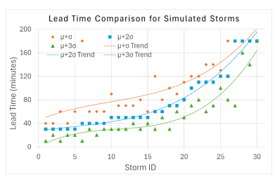
In Figure 12, each marker represents the lead time associated with a single storm event, while the curves indicate the fitted trends. Lead time is limited to the 180-minute detection window prior to storm onset. Several storms exhibit short lead time, particularly under higher thresholds, indicating that higher thresholds tend to delay critical alerts and reduce early warning capability.
Table 3 shows detection performance across 30 simulated storm cases under three anomaly detection thresholds, \mu + \sigma,\ \mu + 2\sigma,\ \text{and}\ \mu + 3\sigma. Precision, recall, and F1 score are reported as mean ± standard deviation, while lead time is reported as the average across all storms. Increasing the threshold from \mu + \sigma,\ \text{to}\ \mu + 3\sigma leads to a substantial improvement in precision, rising from 0.731 to 0.996, indicating a significant reduction in false positives. Recall remains consistently high across all thresholds and reaches 1.000 ± 0.000 at \mu + 3\sigma, showing that all storms are detected with no false negatives. As a result, the F1 score also improves and becomes more stable, with both its mean and variance indicating more consistent performance at higher thresholds.
Table 3: Detection performance for 30 simulated storm cases under different anomaly detection thresholds.
| Threshold | Precision | Recall | F1 Score | Lead Time |
|---|---|---|---|---|
| μ + σ | 0.731 ± 0.298 | 0.981 ± 0.097 | 0.827 ± 0.230 | 103 min |
| μ + 2σ | 0.940 ± 0.139 | 0.987 ± 0.068 | 0.958 ± 0.108 | 78 min |
| μ + 3σ | 0.996 ± 0.017 | 1.000 ± 0.000 | 0.997 ± 0.009 | 52 min |
However, this performance improvement introduces an important operational trade-off. Lower thresholds such as \mu + \sigma provide significantly longer lead times (103 minutes), which are valuable for early warning, but they also exhibit higher false positive rates with greater variability, as reflected in the large standard deviation in precision (±0.298). In contrast, higher thresholds such as \mu + 3\sigma yield highly stable and near-perfect detection performance (precision ±0.017, F1 ±0.009), but at the cost of reduced lead time (52 minutes), potentially limiting the window for proactive response. These results highlight a trade-off between early detection and reliability. Higher thresholds reduce false alarms and provide more consistent detection but may delay warnings. Lower thresholds allow earlier detection but may increase false alarms, requiring additional filtering or decision support. Therefore, threshold selection should depend on application needs, balancing early warning against tolerance for false positives. In this study, the threshold provides a good balance, offering high detection accuracy with reasonable lead time.
Figure 13 shows the anomaly score over time for a representative simulated storm event using a threshold of \mu + 2\sigma\ = 4.085 (\sigma=2/215 and \mu=0.935) This example corresponds to Storm No. 15, with a lead time of 50 minutes. The dashed horizontal line represents the detection threshold, and the vertical gray line indicates the estimated storm onset time. During the normal period, shown in green, the anomaly score stays below the detection threshold and varies within the typical background range. As the simulated storm develops, the anomaly score increases and first crosses the threshold, producing an advisory alert (yellow) that indicates an initial deviation from normal conditions. As the storm intensifies, the anomaly score rises further and remains above the threshold, triggering sustained critical alerts (red). The vertical gray line marks the observed storm onset. The time of the first critical alert corresponds to in Eq. (17), and the lead time is the interval between this alert and the storm onset time tg. In this example, the critical alert occurs before storm onset, showing that the model can detect storm-related anomalies in advance.
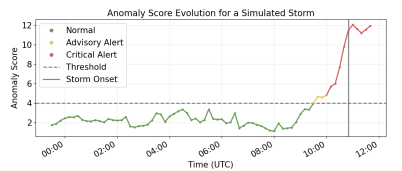
7.2. Performance Evaluation on Real-World Storm Data
To evaluate the proposed method under realistic conditions, we compiled a dataset of 20 historical storm events from the IBTrACS dataset [41]. These events include both rapidly developing storms and gradually intensifying cyclonic disturbances. For each storm, meteorological variables were obtained from the ERA5 reanalysis dataset [14] at hourly resolution on a 0.25° spatial grid and then interpolated to a 10-minute interval.
A key challenge arises from the IBTrACS dataset, which reports storm positions at 3-hour intervals. This coarse resolution makes it difficult to estimate precise lead times. For example, a storm recorded at 12:00 may have begun developing earlier or later within that window. Using the reported time directly can therefore lead to inaccurate lead-time estimates when anomaly detection operates at a higher resolution. To address this, storm onset times were refined using objective meteorological criteria and local atmospheric trends. The onset was defined as the first 10-minute interval within the 3-hour reporting window that satisfies both conditions: wind speed exceeding 11.3 m/s and surface pressure dropping by at least 3 hPa relative to the preceding 12-hour rolling mean. This approach aligns the onset time with observable atmospheric changes in the ERA5 data while remaining consistent with IBTrACS reporting. For each storm, the data were separated into two periods. A background period of about four months before the event was used for training. The test period consisted of the 12 hours before storm onset, sampled at 10-minute intervals, capturing the formation phase. An autoencoder was trained on the background data and then applied to the test period to detect anomalous behavior before or during storm development. The results show that the model consistently identified anomalies in real-world storms prior to storm intensification.
Figure 14 shows the lead times for the 20 real storm events under three anomaly detection thresholds: 7.2.Performance Evaluation on Real-World Storm Data
To evaluate the proposed method under realistic conditions, we compiled a dataset of 20 historical storm events from the IBTrACS dataset [41]. These events include both rapidly developing storms and gradually intensifying cyclonic disturbances. For each storm, meteorological variables were obtained from the ERA5 reanalysis dataset [14] at hourly resolution on a 0.25° spatial grid and then interpolated to a 10-minute interval.
A key challenge arises from the IBTrACS dataset, which reports storm positions at 3-hour intervals. This coarse resolution makes it difficult to estimate precise lead times. For example, a storm recorded at 12:00 may have begun developing earlier or later within that window. Using the reported time directly can therefore lead to inaccurate lead-time estimates when anomaly detection operates at a higher resolution. To address this, storm onset times were refined using objective meteorological criteria and local atmospheric trends. The onset was defined as the first 10-minute interval within the 3-hour reporting window that satisfies both conditions: wind speed exceeding 11.3 m/s and surface pressure dropping by at least 3 hPa relative to the preceding 12-hour rolling mean. This approach aligns the onset time with observable atmospheric changes in the ERA5 data while remaining consistent with IBTrACS reporting. For each storm, the data were separated into two periods. A background period of about four months before the event was used for training. The test period consisted of the 12 hours before storm onset, sampled at 10-minute intervals, capturing the formation phase. An autoencoder was trained on the background data and then applied to the test period to detect anomalous behavior before or during storm development. The results show that the model consistently identified anomalies in real-world storms prior to storm intensification.
Figure 14 shows the lead times for the 20 real storm events under three anomaly detection thresholds: μ+σ, μ+2σ, and μ+3σ, derived from fair-weather observations. Each marker represents the lead time for one storm, while the fitted curves show the overall trend for each threshold. Lead time values are capped at the 180-minute operational detection window. derived from fair-weather observations. Each marker represents the lead time for one storm, while the fitted curves show the overall trend for each threshold. Lead time values are capped at the 180-minute operational detection window.
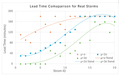
As shown in Figure 14, the detection threshold strongly influences storm alert performance. Lower thresholds tend to produce earlier detections, resulting in longer lead times across most storms. Conversely, higher thresholds delay anomaly detection and reduce lead time. The spread of points across storms indicates variability in storm development, leading to different detection times even under the same threshold. The trend lines highlight this systematic effect:
As shown in Figure 14, the detection threshold strongly influences storm alert performance. Lower thresholds tend to produce earlier detections, resulting in longer lead times across most storms. Conversely, higher thresholds delay anomaly detection and reduce lead time. The spread of points across storms indicates variability in storm development, leading to different detection times even under the same threshold. The trend lines highlight this systematic effect: \mu + \sigma, produces the earliest warnings, often approaching the upper limit of the detection window, whereas \mu + 3\sigma yields sho \mu + 2\sigma,\ falls between these extremes, indicating a balance between early detection and reduced false alerts.
Table 4 presents detection performance for the 20 real storm cases under three anomaly detection thresholds, \mu + \sigma,\ \mu + 2\sigma,\ \text{and}\ \mu + 3\sigma. Precision, recall, and F1 score are reported as mean ± standard deviation, while lead time is reported as the average across all storms. Compared to the simulated results, performance on real storm data exhibits greater variability, reflecting the increased complexity and noise in real-world atmospheric conditions. As the threshold increases from \mu + \sigma, \text{to}\ \mu + 3\sigma, precision improves from 0.526 to 0.892, indicating fewer false positives. However, unlike the simulated setting, recall decreases from perfect detection (1.000 ± 0.000) at \mu + \sigma,\ to \mu + 3\sigma 0.963 ± 0.116 at , suggesting that stricter thresholds may introduce false negatives. The F1 score reflects this trade-off, increasing from 0.615 to 0.910, indicating a better balance between precision and recall at higher thresholds despite the slight drop in recall.
Table 4: Detection performance for 20 real storm cases under three different anomaly detection thresholds.
| Threshold | Precision | Recall | F1 Score | Lead Time |
|---|---|---|---|---|
| μ + σ | 0.526 ± 0.192 | 1.000 ± 0.000 | 0.615 ± 0.167 | 155 min |
| μ + 2σ | 0.832 ± 0.182 | 0.997 ± 0.010 | 0.892 ± 0.142 | 114 min |
| μ + 3σ | 0.892 ± 0.209 | 0.963 ± 0.116 | 0.910 ± 0.190 | 69 min |
produces the earliest warnings, often approaching the upper limit of the detection window, whereas yields shorter lead times for most storms. The intermediate threshold falls between these extremes, indicating a balance between early detection and reduced false alerts.
Table 4 presents detection performance for the 20 real storm cases under three anomaly detection thresholds, , , and . Precision, recall, and F1 score are reported as mean ± standard deviation, while lead time is reported as the average across all storms. Compared to the simulated results, performance on real storm data exhibits greater variability, reflecting the increased complexity and noise in real-world atmospheric conditions. As the threshold increases from to , precision improves from 0.526 to 0.892, indicating fewer false positives. However, unlike the simulated setting, recall decreases from perfect detection (1.000 ± 0.000) at to 0.963 ± 0.116 at , suggesting that stricter thresholds may introduce false negatives. The F1 score reflects this trade-off, increasing from 0.615 to 0.910, indicating a better balance between precision and recall at higher thresholds despite the slight drop in recall.
The standard deviations further highlight variability across storms, particularly at higher thresholds (e.g., precision \mu + 3\sigma ±0.209 at ), suggesting that performance is more sensitive to storm characteristics and environmental conditions in real data. A clear trade-off is also observed in lead time. Lower thresholds provide earlier warnings (155 minutes at \mu + \sigma,\) but with lower precision and higher variability. Higher thresholds yield more reliable alerts but reduce lead time (69 minutes at \mu + 3\sigma), potentially limiting response time. The intermediate threshold offers a balanced operating point, achieving high recall (0.997), strong precision (0.832), and a moderate lead time (114 minutes), making it a practical choice for real-world deployment. Overall, these results show that while sigma-based thresholds generalize well to real-world conditions, the trade-off between lead time and reliability becomes more pronounced, and threshold selection should be guided by application-specific requirements.
Figure 15 shows a representative real storm case (Storm No. 6), illustrating the temporal evolution of the anomaly score before storm onset. An anomaly detection threshold of \mu + 2\sigma\ = 4.272 (\sigma=2.564 and \mu=0.864) is used, resulting in a lead time of 60 minutes. The dashed horizontal line represents the threshold separating normal and abnormal atmospheric behavior, while the vertical gray line marks the estimated storm onset.
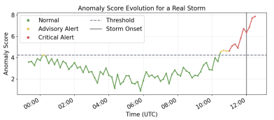
As shown in Figure 15, during the early period, the anomaly score remains below the threshold and is classified as normal behavior (green). As the storm develops, the anomaly score increases and first exceeds the threshold, producing advisory alerts (yellow). As conditions intensify, the anomaly score rises further and enters the critical alert region (red). The anomaly score shows a sustained increase during storm formation, reaching a peak shortly before the onset. This behavior demonstrates that the model detects abnormal patterns in advance. The progression from normal conditions to advisory and then critical alerts illustrates the system’s ability to provide early warning during storm development process.
8. Conclusions and Future Work
This study presents an unsupervised anomaly detection framework for the early identification of maritime storm formation using autoencoders trained on multivariate meteorological time-series data. The proposed approach relies exclusively on locally measurable atmospheric variables, allowing the system to operate without satellite or radar observations. This design makes the framework suitable for deployment on vessels operating in remote ocean regions, including ships with limited access to large-scale monitoring infrastructure. The framework was evaluated using both simulated storm scenarios and historical storm events derived from the IBTrACS dataset [41], together with meteorological fields from the ERA5 reanalysis dataset [14]. Experimental results show that the autoencoder consistently detects abnormal atmospheric behavior during the storm formation phase. Across both synthetic and real storm cases, the system provides early warnings with average lead times exceeding one hour while maintaining reasonable detection accuracy. These findings demonstrate that monitoring reconstruction errors of locally observed atmospheric variables can reveal detectable precursors of storm development before the storm is fully formed. The framework therefore provides a lightweight and effective mechanism for real-time storm detection and offers a promising step toward autonomous early-warning capabilities for maritime safety.
Future work will focus on improving both interpretability and operational applicability. Explainable artificial intelligence methods, such as SHAP (SHapley Additive exPlanations) [42], will be incorporated to better understand how individual meteorological variables contribute to anomaly detection. Such analysis can enhance operator confidence and help distinguish genuine storm precursors from anomalies caused by sensor noise or unrelated atmospheric variability. In addition, the framework will be extended to support regional or basin-level models, enabling generalization across broader geographic environments and large-scale atmospheric dynamics [14, 43]. Future studies will incorporate additional real-world storm events from diverse geographic regions and multiple storm categories to evaluate the robustness and generalizability of the proposed framework under varying environmental and climatic conditions. Finally, further validation will be conducted using high-frequency shipboard sensor measurements to assess performance under real operational conditions. These developments will help advance the proposed approach toward practical deployment for onboard storm monitoring and early warning in maritime environments.
- FAO, “Fatalities in Fisheries,” Document X9656E, Food and Agriculture Organization (FAO) of the United Nations, 2025. Available online: https://www.fao.org/4/x9656e/X9656E.htm (accessed on July 1, 2025).
- PRC, “More Than 100,000 Fishing-Related Deaths Occur Each Year, Study Finds,” Pew Research Center (PRC), The Pew Charitable Trusts, November 2022. Available online: https://www.pew.org/-/media/assets/2022/12/fisher-mortality-brief-v3.pdf (accessed on July 1, 2025).
- WMO, “Global Observing System (GOS),” World Meteorological Organization (WMO) of the United Nations, 2025. Available online: https://wmo.int/activities/global-observing-system-gos/global-observing-system-gos (accessed on July 1, 2025).
- NOAA, “National Hurricane Center and Central Pacific Hurricane Center,” National Oceanic and Atmospheric Administration (NOAA), 2025. Available online: https://www.nhc.noaa.gov/ (accessed on July 1, 2025).
- S. R. Smith, “Ship-based Contributions to Global Ocean, Weather, and Climate Observing Systems,” Frontiers in Marine Science, vol. 6, article 434, 2019, doi: 10.3389/fmars.2019.00434.
- EMSA, “Annual Overview of Marine Casualties and Incidents,” European Maritime Safety Agency (EMSA), 2024. Available online: https://www.emsa.europa.eu/publications/item/5352-annual-overview-of-marine-casualties-and-incidents-2024.html (accessed on July 1, 2025).
- National Research Council, Opportunities to Improve Marine Forecasting. Washington, DC, USA: The National Academies Press, 1989, doi: 10.17226/1410.
- M. Nazarihaghighipashaki, B. E. Moen, and M. Bratveit, “Fatal Occupational Injuries in Fishing, Farming and Forestry 2010–2015,” Occupational Medicine, vol. 74, no. 7, pp. 523–529, October 2024, doi: 10.1093/occmed/kqae073.
- WMO, Global Guide to Tropical Cyclone Forecasting, WMO-No. 1194, Geneva: World Meteorological Organization (WMO), 2017. Available online: https://cyclone.wmo.int/pdf/Global-Guide-to-Tropical-Cyclone-Forecasting.pdf (accessed on July 1, 2025).
- P. Bauer, A. Thorpe, and G. Brunet, “The quiet revolution of numerical weather prediction,” Nature, vol. 525, pp. 47–55, 2015, doi: 10.1038/nature14956.
- J. R. Holton and G. J. Hakim, An Introduction to Dynamic Meteorology, 5th ed. Waltham, MA, USA: Academic Press, 2013.
- C. L. Loi, C.-C. Wu, and Y.-C. Liang, “Prediction of tropical cyclogenesis based on machine learning methods and its SHAP interpretation,” Journal of Advances in Modeling Earth Systems, vol. 16, no. 3, pp. 1–20, March 2024, doi: 10.1029/2023MS003637.
- C. Kieu and Q. Nguyen, “Binary dataset for machine learning applications to tropical cyclone formation prediction,” Scientific Data, vol. 11, article no. 446, pp. 1–10, May 2024, doi: 10.1038/s41597-024-03281-5.
- H. Hersbach, B. Bell, P. Berrisford, S. Hirahara, A. Horányi, J. Muñoz-Sabater, J. Nicolas, C. Peubey, R. Radu, D. Schepers, et al., “The ERA5 global reanalysis,” Quarterly Journal of the Royal Meteorological Society, vol. 146, no. 730, pp. 1999–2049, May 2020, doi: 10.1002/qj.3803.
- D. Fan, S. J. Greybush, E. E. Clothiaux, and D. J. Gagne, “Physically explainable deep learning for convective initiation nowcasting using GOES-16 satellite observations,” Artificial Intelligence for the Earth Systems, vol. 3, e230098, 2024, doi: 10.1175/AIES-D-23-0098.1.
- B. Tong, G. Hu, and Z. Duan, “Transformer-based full-track simulation of tropical cyclones,” Journal of Wind Engineering and Industrial Aerodynamics, vol. 265, article no. 106176, 2025, doi: 10.1016/j.jweia.2025.106176.
- W. Girard, H. Xu, and D. Yan, “SeADL: self-adaptive deep learning for real-time marine visibility forecasting using multi-source sensor data,” Sensors, vol. 26, no. 2, article no. 676, pp. 1–28, 2026, doi: 10.3390/s26020676.
- V. Chandola, A. Banerjee, and V. Kumar, “Anomaly detection: a survey,” ACM Computing Surveys, vol. 41, no. 3, article 15, pp. 1–58, July 2009, doi: 10.1145/1541880.1541882.
- J. J. Downs and E. F. Vogel, “A plant-wide industrial process control problem,” Computers & Chemical Engineering, vol. 17, no. 3, pp. 245–255, 1993.
- Q. Cheng, K. Hong, K. Huang, and Z. Liu, “Evaluating effectiveness and identifying appropriate methods for anomaly detection in intelligent transportation systems,” IEEE Transactions on Intelligent Transportation Systems, vol. 26, no. 8, pp. 11442–11453, Aug. 2025, doi: 10.1109/TITS.2025.3580960.
- T. Inaba, “Supply chain anomaly detection by using simulation and machine learning,” in Proceedings of the 2025 IEEE International Conference on Industrial Engineering and Engineering Management (IEEM), Melbourne, Australia, December 7–10, 2025, pp. 6–10, doi: 10.1109/IEEM63636.2025.11357657.
- G. Pang, C. Shen, L. Cao, and A. V. D. Hengel, “Deep learning for anomaly detection: a review,” ACM Computing Surveys, vol. 54, no. 2, article 38, pp. 1–38, March 2022, doi: 10.1145/3439950.
- G. Zhu, H. Zhao, H. Liu, and H. Sun, “A novel LSTM-GAN algorithm for time series anomaly detection,” in Proceedings of the 2019 Prognostics and System Health Management Conference (PHM-Qingdao), Qingdao, China, 2019, pp. 1–6, doi: 10.1109/PHM-Qingdao46334.2019.8942842.
- M. R. Fachrezi, A. F. Ihsan, and W. Astuti, “Anomaly detection using LSTM-based deep learning on natural gas pipeline operational data,” in Proceedings of the 2024 12th International Conference on Information and Communication Technology (ICoICT), Bandung, Indonesia, August 7–8, 2024, pp. 500–506, doi: 10.1109/ICoICT61617.2024.10698714.
- M. Du, F. Li, G. Zheng, and V. Srikumar, “DeepLog: anomaly detection and diagnosis from system logs through deep learning,” in Proceedings of the 2017 ACM SIGSAC Conference on Computer and Communications Security (CCS ’17), Association for Computing Machinery, New York, NY, USA, pp. 1285–1298, 2017, doi: 10.1145/3133956.3134015.
- Y. Su, Y. Zhao, C. Niu, R. Liu, W. Sun, and D. Pei, “Robust anomaly detection for multivariate time series through stochastic recurrent neural network,” in Proceedings of the 25th ACM SIGKDD International Conference on Knowledge Discovery & Data Mining (KDD ’19), Association for Computing Machinery, New York, NY, USA, pp. 2828–2837, 2019, doi: 10.1145/3292500.3330672.
- S. Tuli, G. Casale, and N. R. Jennings, “TranAD: deep transformer networks for anomaly detection in multivariate time series data,” in Proceedings of the VLDB Endowment, vol. 15, no. 6, pp. 1201–1214, 2022, doi: 10.14778/3514061.3514067.
- K. Berahmand, F. Daneshfar, E. S. Salehi, Y. Li, and Y. Xu, “Autoencoders and their applications in machine learning: a survey,” Artificial Intelligence Review, vol. 57, article no. 28, 2024, doi: 10.1007/s10462-023-10662-6.
- S. Givnan, C. Chalmers, P. Fergus, S. Ortega-Martorell, and T. Whalley, “Anomaly detection using autoencoder reconstruction upon industrial motors,” Sensors, vol. 22, no. 9, p. 3166, Apr. 2022, doi: 10.3390/s22093166.
- S. Ahmad, K. Styp-Rekowski, S. Nedelkoski, and O. Kao, “Autoencoder-based condition monitoring and anomaly detection method for rotating machines,” in Proceedings of the 2020 IEEE International Conference on Big Data (Big Data), Atlanta, GA, USA, pp. 4093–4102, 2020, doi: 10.1109/BigData50022.2020.9378015.
- T.-W. Tang, W.-H. Kuo, J.-H. Lan, C.-F. Ding, H. Hsu, and H.-T. Yang, “Anomaly detection neural network with dual auto-encoders GAN and its industrial inspection applications,” Sensors, vol. 20, no. 12, article no. 3336, 2020, doi: 10.3390/s20123336.
- P. Malhotra, A. Ramakrishnan, G. Anand, L. Vig, P. Agarwal, and G. Shroff, “LSTM-based encoder-decoder for multi-sensor anomaly detection,” in Proceedings of the ICML 2016 Anomaly Detection Workshop, New York, NY, USA, June 24, 2016, doi: 10.48550/arXiv.1607.00148.
- T. Kim, J. Kim, and I. You, “An anomaly detection method based on multiple LSTM-autoencoder models for in-vehicle network,” Electronics, vol. 12, no. 17, article no. 3543, pp. 1–17, 2023, doi: 10.3390/electronics12173543.
- F. M. Bianchi, L. Livi, K. Mikalsen, M. Kampffmeyer, and R. Jenssen, “Learning representations of multivariate time series with missing data,” Pattern Recognition, vol. 96, article no. 106973, 2019, doi: 10.1016/j.patcog.2019.106973.
- G. Pallotta, M. Vespe, and K. Bryan, “Vessel pattern knowledge discovery from AIS data: a framework for anomaly detection and route prediction,” Entropy, vol. 15, no. 6, pp. 2218–2245, 2013, doi: 10.3390/e15062218.
- T. T. Fujita, The Downburst: Microburst and Macroburst, Project Report, Satellite and Mesometeorology Research Project (SMRP), Department of Geophysical Sciences, University of Chicago, Chicago, IL, USA, 1985.
- T. M. Weckwerth, “The effect of small-scale moisture variability on thunderstorm initiation,” Monthly Weather Review, vol. 128, no. 12, pp. 4017–4030, December 2000, doi: 10.1175/1520-0493(2000)129<4017:TEOSSM>2.0.CO;2.
- R. J. Small, S. P. de Szoeke, S. P. Xie, L. O’Neill, H. Seo, Q. Song, P. Cornillon, M. Spall, and S. Minobe, “Air–sea interaction over ocean fronts and eddies,” Dynamics of Atmospheres and Oceans, vol. 45, no. 3–4, pp. 274–319, August 2008, doi: 10.1016/j.dynatmoce.2008.01.001.
- L. H. Holthuijsen, Waves in Oceanic and Coastal Waters. Cambridge, U.K.: Cambridge University Press, 2007.
- J. J. Jensen, A. E. Mansour, and A. S. Olsen, “Estimation of ship motions using closed-form expressions,” Ocean Engineering, vol. 31, no. 1, pp. 61–85, 2004, doi: 10.1016/S0029-8018(03)00108-2.
- K. R. Knapp, M. C. Kruk, D. H. Levinson, H. J. Diamond, and C. J. Neumann, “The international best track archive for climate stewardship (IBTrACS): unifying tropical cyclone best track data,” Bulletin of the American Meteorological Society, vol. 91, no. 3, pp. 363–376, 2010, doi: 10.1175/2009BAMS2755.1.
- S. M. Lundberg and S.-I. Lee, “A unified approach to interpreting model predictions,” in Proceedings of the 31st International Conference on Neural Information Processing Systems (NIPS ’17), Curran Associates Inc., Red Hook, NY, USA, pp. 4768–4777, 2017.
- K. Bi, L. Xie, H. Zhang, X. Chen, X. Gu, and Q. Tian, “Accurate medium-range global weather forecasting with 3D neural networks,” Nature, vol. 619, pp. 533–538, 2023, doi: 10.1038/s41586-023-06185-3.